I am thinking about moving this discussion about QUBOs to its own tab as we are kinda in a constant thread of thought talking about QUBO problems. In this post, I want to talk about how we can upgrade our persistence results that we derived in the second QUBO post to be even more powerful by taking ideas from the post about shifting out problems. I will leave many manipulations at the bottom if you are interested, but I will not muddle the narrative too much by doing a bunch of algebra. And a relatively simple step of removing the fixed variables from the subproblems we are solving, as we already know they are fixed, allows us to reduce the difficulty of the subproblems we are solving.
Proving that more Variables are Fixed
\[\begin{align} f(x) &= \frac{1}{2}x^TQx + c^Tx\\ f_\mu(x) &= \frac{1}{2}x^T(Q - \text{diag}\{u\})x + (c+0.5u)^Tx \end{align}\]Now to review what the persistency results say, if we can show for any realization of $x\in{0,1}^n$ that $\nabla_i f(x) \leq 0$ then $x_i = 1$ and similarly for the case where $\nabla_i f(x) \geq 0$ then $x_i = 0$. So this naturally begs the question, can we make an equivalent $f_\mu(x)$ such that we can force this to happen or at the least tighten the bounds of $\nabla f_\mu(x)$ to be tight? The answer is yes, and the particular value of this shift is quite easy to compute, actually in $\mathcal{O}(n)$ time. First, we will start with how the function gradient changes w.r.t. $u$.
\[\begin{align} \nabla_x f(x) &= Qx + c\\ \nabla_x f_u(x) &= Qx + \text{diag}\{u\}x - 0.5u + c \end{align}\]Given this, we can express the lower and upper bounds of each gradient component as a function of $u$. Where $\lambda_i$ and $\upsilon_i$ are constants and not a function of $u$. Both have their maximum/minimum respectively at $u_i = -Q_{i,i}$.
\[\begin{align} \min_{x \in \{0,1\}^N} \nabla_xf^i_\mu(x) &= \min\{Q_{i,i} + u_i, 0\} -0.5u_i + \lambda_i\\ \max_{x \in \{0,1\}^N} \nabla_xf^i_\mu(x) &= \max\{Q_{i,i} + u_i, 0\} - 0.5u_i + \upsilon_i \end{align}\]So, to calculate the $u$ that brings in the bounds of the gradients of the QUBO the most, we can set it equal to the negative diagonal of $Q$. Bringing this back to the application, when preprocessing the QUBOs, we need to more or less rewrite the $\alpha x_i^2$ terms as $0.5\alpha x_i$ terms. By doing so, we can run the persistency checks on this transformed function, and it will be able to identify a (hopefully) larger set of variables as fixed.
A consequence of this is that all instances of diagonal problems are now solved in the resolve phase. So, there is now a richer class of problems that we can solve exactly without branching and bounding. In the future, it might make sense for me to implement special structure identification for cases of QUBO where there are known fast algorithms or shortcuts, such as known polynomial solutions for tridiagonal problems.
Reducing Subproblem size
This step is more or less self explanatory in that if we already know that we have fixed a set of variables $x_i = p_i, \quad \forall i \in \mathcal{I}$, then we can remove them from the optimization formulation entirely by substitution the values directly into the function $f(x)$.
\[\begin{align} \min_{x\in\{0,1\}^n} &\frac{1}{2}x^TQx + c^Tx\\ \text{s.t. } x_i &= p_i, \quad \forall i \in \mathcal{I}\\ 0 \leq &x_j \leq 1, \quad \forall j \in \{1,\dots,n\} \end{align}\]This lets us project our subproblem into a smaller variable space.
\[\begin{align} \min_{\hat{x}\in\{0,1\}^{n - |\mathcal{I}|}} &\frac{1}{2}\hat{x}^T\hat{Q}\hat{x} + \hat{c}^T\hat{x}\\ \text{s.t. } 0 \leq &\hat{x}_j \leq 1, \quad \forall j \in \{1,\dots,n - |\mathcal{I}|\} \end{align}\]Benchmarking
I guess this is getting somewhat cliched, in basically every single post in this series is more or less “Here is an idea” than “Let’s see if it made it faster”. But we will be repeating this here. We will check the effects of these two changes in tandem without using the SDP tightening on the same set of problems in the last post, e.g., 50 problems with 75 variables and a density of approximately 10%. The code to generate the problem set can be seen at the post’s bottom.
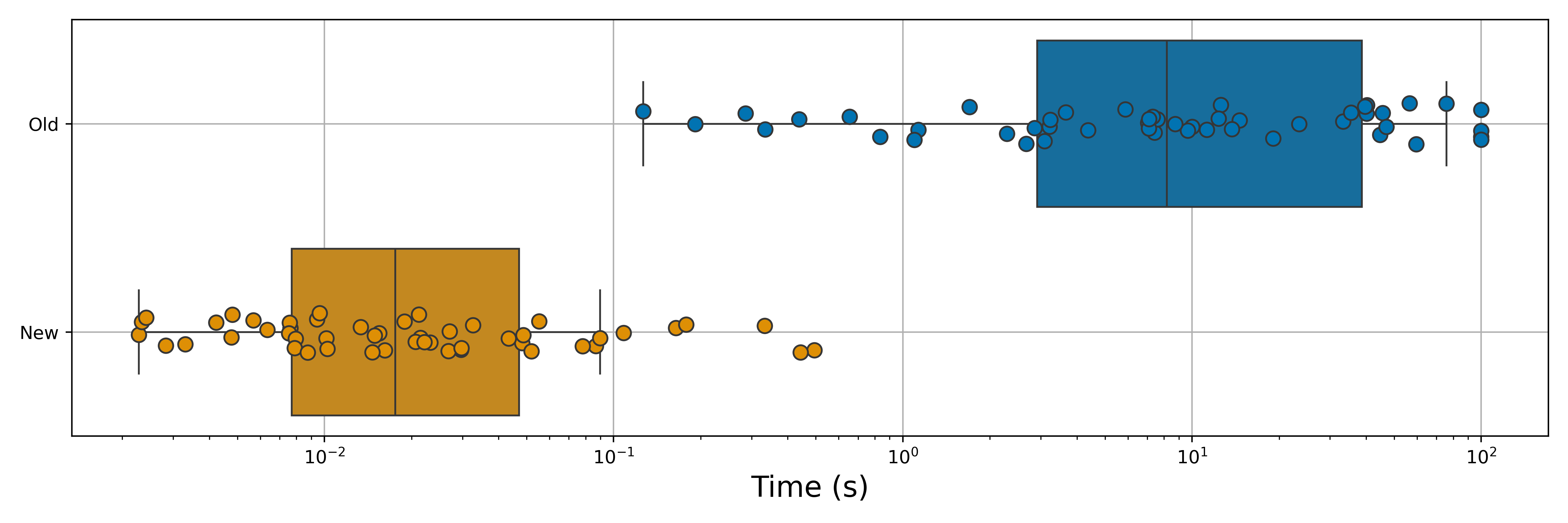
As we can see, this greatly reduces the solve times. This is primarily due to the preprocessor being able to fix many variables from the start that raise the lower bound of the QP relaxation (as well as fixing more along). But we can see that we have reduced our median time to solve by approximately a factor of 400 by utilizing this new resolve and subproblem reduction approach. Not too bad!
Looking forward, it makes sense to start applying cuts or domain propagation methods that have been applied in the literature before to strengthen each node. For the human side of things, it would be nice to start adding a modeling interface so that people can start writing optimization models in a more ‘human’ method similar to what people do in pyomo or gurobipy. A few more tricks can be pulled off via preprocessing, but those need more architecture that comes naturally from a cut-and-branch (or branch-and-cut) scheme, so I don’t know when I will add this.
Math Appendix
The expression for the gradient of our transformed function.
\[\begin{align} \nabla_x f^i_u(x) &= Q_ix + u_ix_i - 0.5u_i + c_i\\ &= (Q_{i,i} + u_i)x_i + c_i - 0.5\mu +\sum_{j \in N\setminus i} Q_{i,j}x_j \end{align}\]How the minimum and maximum $i^{\text{th}}$ component of the vector of $\nabla_x f_u(x)$ can be computed.
\[\begin{align} \min_{x \in \{0,1\}^N} \nabla_xf^i_u(x) &= \min\{(Q_{i,i} + u_i)x_i,0\} + c_i - 0.5u_i +\sum_{j \in N\setminus i} \min\{Q_{i,j}x_j , 0\}\\ &=\min\{Q_{i,i} + u_i, 0\} + c_i -0.5u_i + \sum_{j \in N\setminus i} \min\{Q_{i,j},0\}\\ &=\min\{Q_{i,i} + u_i, 0\} -0.5u_i + \lambda_i\\ \max_{x \in \{0,1\}^N} \nabla_xf^i_u(x) &= \max\{(Q_{i,i} + u_i)x_i,0\} + c_i - 0.5u_i +\sum_{j \in N\setminus i} \max\{Q_{i,j}x_j , 0\}\\ &=\max\{Q_{i,i} + u_i, 0\} + c_i -0.5u_i + \sum_{j \in N\setminus i} \max\{Q_{i,j},0\}\\ &= \max\{Q_{i,i} + u_i, 0\} - 0.5u_i + \upsilon_i \end{align}\]Code
def make_random_var(n:int):
    return numpy.random.rand(n)-0.5

def generate_problem(problem_id: int):
    numpy.random.seed(1696979520 + problem_id)
    N = 75
    Q = sp.random(N, N, 0.05, format = 'csr', data_rvs=make_random).todense()
    Q = numpy.array(Q)
    Q = 0.5*(Q.T + Q) # Q ~ 10% dense
    c = numpy.random.rand(N,1) - 0.5

    # convexify the QUBO
    f = min(numpy.linalg.eigvalsh(Q))

    Q = Q - f*numpy.eye(N)
    c = c + 0.5*f

    return QUBOProblem(Q, c)

problems = [generate_problem(id).herc_rep for id in range(50)]
warm_starts = [hercules.pso(p,123456,10, 100)[0] for p in problems]

def bench_problem(prob, start):
    return hercules.solve_branch_bound(prob, 100, warm_start=start, threads = 1025, branch_strategy='WorstApproximation')[2]


solve_times = [bench_problem(prob, start) for prob, start in zip(problems, warm_starts)]