Branch And Bound of QUBO, Using Heuristics

This is a follow up post to one I made last October, where we made a very simple branch and bound solver for solving QUBO problems. Here we are going to see the effect of adding some concepts from the heuristics literature to speed up finding the global optimum of the problem. Roughly speaking, we can use near optimal solutions we find from heuritsics to give us much better initial bounds, allowing us to prune from the branch and bound tree faster. Additionally, we can use some problem specific properties to reduce the number of variables we actually branch on, from a property known as persistancy. We still won’t improve the branching rules or node selection stratagy, we will leave this for another day. I mostly want to point out the large jump in performance we get when we incorperate a better initial point and a problem specific stratagy to cut down to number of variables we need to look at. As a reminder we are looking at the following problem.

Heuristics for an initial solution

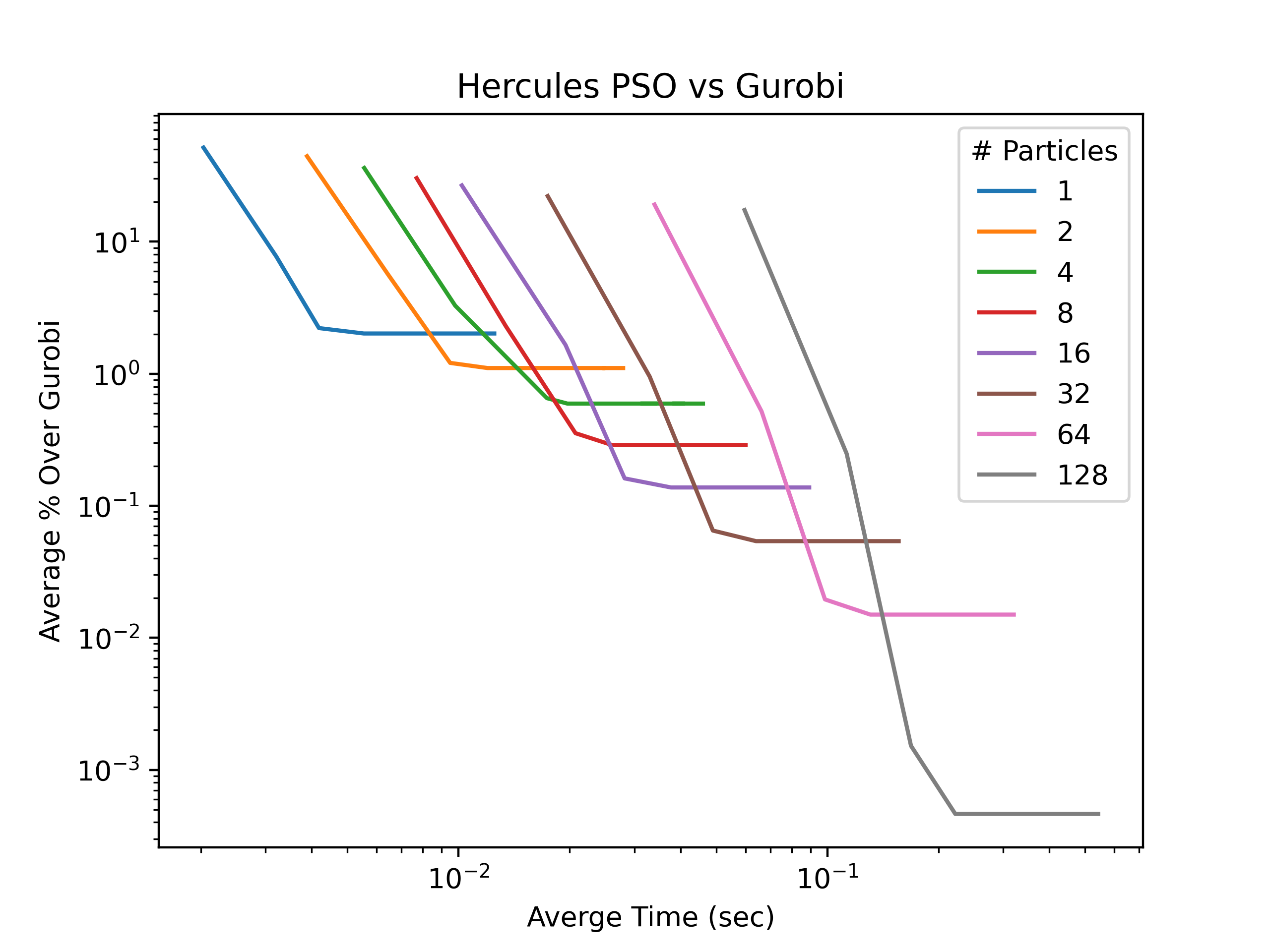
Roughly speaking, we find approximate solutions to reduce the number of nodes in the branch and bound tree that we have to explore. I wrote a package for heuristics on QUBO problems, called hercules, it is open source and written in Rust so it is quite fast. I will be using this to generate initial solutions for all of the tests. Currently, to use it in python you need to build it using maturin develop. It performs quite well, in finding optimal solutions, especially when compaired to commerical tools, such as Gurobi. Here, we can look at the comparison of Gurobi with using the particle swarm optimization (PSO) algorithm. Here we are comparing Gurobi 11.0 given 5 seconds to find heuristic solutions and try to solve, vs. hercules with PSO. This is based on 100 nonconvex QUBO problem instances generated, and looks at the averages of how long it took to solve and compares to the. There is not an instance where PSO finds better solutions then Gurobi, but thy typically find the same solution with some problem instances giving nearly as good solutions.

To modify the previous code to work with hercules, we add the following function to the QUBOProblem class. This generates data in the format that hercules expects the problem data in.

class QUBOProblem:

    def make_hercules_rep(self):
        i_coords = []
        j_coords = []
        q_vals = []
        for i in range(self.num_x()):
            for j in range(self.num_x()):
                if self.Q[i,j] != 0.0:
                    i_coords.append(i)
                    j_coords.append(j)
                    q_vals.append(self.Q[i,j])
        c_vals = [self.c[i,0] for i in range(self.num_x())]
        return (i_coords, j_coords, q_vals, c_vals, self.num_x())

In this example we will use the particle swarm algorithm to find a good initial point. This can be accomplished with the following python code. We get an initial guess

# where p is a QUBOProblem
problem_data = p.make_hercules_rep()

seed = int(time.time())
num_iters = 50
num_particales = 10

# run particle swarm optimization
# x_0 is the best solution found, obj is the objective
x_0, obj = hercules.pso(prob_data, seed, num_particales, num_iters)

As the code from the previous post already can accept an initial solution, we do not have to do further modifications to pass this solution to the solver we have been making.

Persistancy to Fix Variables

A well known results in the QUBO literature is known as persistancy. What persistancy is that, given the certain bounds on the gradient of a convex QUBO (or QUBO that has been made convex), we can state ahead of time, that the solution must have certain variables fixed. This allows for us to reduce the number of variables that we have to solve for and has to potential to massively reduce the size of the search space. For example, in a worst case senario, where we need to look at all possible combinations, if we have 20 variables that need to be solved vs 10, we need to look at 1024x more nodes. In the situation where, we have already found the optimal solution, but need to prove it, this is a huge help in cutting down the decision space.

To get more clear with how we find if a variable is persistant, we apply the following check

With this, we know if $x_i$ is fixed at 1 or 0, which means that this is removed from the branching choices. This can be solved in linear time for each variable, $O(n)$ at worst, so a full pass for each variable is $O(n^2)$. We would want to repeat this process up to $n$ times to make sure that we have found each fixed variable so in the worse case we have $O(n^3)$ for the run time of the problem. This is true only when we have dense matrices, in the case of sparse matrices we have a much lower bound of $O(nnz(Q)n)$. The code to do this is implimented in hercules, so I will not show the implimentation here. However, I will show how to call it and integrate it into the solver we have been making.

First we need to actually call it to get the fixed variables. This is simple enough.

# given the same problem_data from the PSO section
persist = hercules.get_persistent_variables(problem_data)

Now, in the last post we didn’t have the functionality of passing a set of fixed variables, this can be fixed by chaning the constructor of the QUBO_solver class slightly.

class QUBO_solver:
    
    def __init__(self, problem, sub_problem_solver, branch_strat, node_strat, initial_sol = None, initial_fixed = None):
        
        if initial_sol is None:
            initial_sol = numpy.zeros(problem.num_x()).reshape(-1,1)
        
        self.problem = problem
        self.initial_sol = initial_sol
        self.initial_bound = self.problem.eval_obj(self.initial_sol)
        self.sub_problem_solver = sub_problem_solver
        self.root = BBNode(self.problem, fixed=initial_fixed)
        self.node_list = [self.root]
        self.checked_nodes = 0
        self.current_upper_bound = self.initial_bound
        self.best_feasible_sol = self.initial_sol
        self.branch_strat = branch_strat
        self.node_strat = node_strat

Basically the only thing that changed is that we are now allowing for passing a dictionary of fixed variables to the solver, and making the root node start with these fixed variables.

Lets see how it works out

We did all of this fancy stuff, but lets see if it actually does anything in solve time. Remember we are doing random node and branch selection, with a quite bad subproblem solver. If we compare to the last post without heuristics, we had to solve about 4000 subproblems. If we incorperate PSO for initil guess calculations, and use the persistancy of variables to reduce the space we only have to solve 51 subproblems, and on my laptop the total elapsed time is now $.002$ seconds. Which is a enormous boost in solve time compared to the previous post. If we only turn off the initial guess it solves in 171 subproblems, and if we only turn of persistancy we solve in 1205 suprobem solves. So these can work together in tandem.

import numpy
import time
import copy
import hercules

N = 20
numpy.random.seed(1696979520)
Q = numpy.random.randn(N,N)/20
Q = Q.T@Q + numpy.eye(N)
c = numpy.random.randn(N).reshape(-1,1)
p = QUBOProblem(Q, c)

prob_data = p.make_hercules_rep()


x_0, obj = hercules.pso(prob_data, 1696979520, 10, 200)
x_0 = numpy.array(x_0).reshape(-1,1)

persist = hercules.get_persistent_variables(prob_data)

qubo_solver = QUBO_solver(p, solve_eq_qp, random_branch_strat,random_node_strat, initial_sol = x_0, initial_fixed=persist)
qubo_solver.solve()