I have been looking at a financial application to optimization; they are fairly interesting and not something that I have seen before. My research is mainly focused on the control, scheduling, and design of physical assets, not financial assets. So I took a stab at solving the classical Markowitz Portfolio optimization problem via multiparametric programming. I chose to do this as it aligns with my research interests (multiparametric programming rise up!). Using multiparametric programming, we extract an explicit form of the optimal Pareto front between risk and return.
The Markowitz portfolio optimization problem is given as follows, where $\Sigma$ is the covariance of the commodities. In this example, we are considering only positive definite covariance matrices. $R^* $ is the return we wish to get, $\mu$ is the expected rate of return. The constraints are effectively specifying a return rate that we want, saying that the composition of our portfolio must sum to one (we only have one portfolio!) and that we can’t have negative positions in any commodity.
\[\begin{align} \min \frac{1}{2} w^T & \Sigma w\\ \sum \mu_i w_i &=R^* \\ \sum w_i &= 1\\ w_i &\geq 0, \forall i \end{align}\]This can be reformulated into an mpQP, or to say we can solve this for all possible realizations of our desired return and recover the Pareto front by switching out $R^* $ with an uncertain parameter $\theta$. Since there is only one uncertain dimension, the geometric algorithm is the most efficient for this problem, and even portfolios with hundreds of commodities can be solved in seconds. However since, trying to plot the optimal portfolio positions for hundreds of commodities, we instead are going to solve it for five commodities so we can still see what is happening under the hood.
Here the covariance matrix and the return coefficients were generated from random numbers as I do not have easy access to this sort of data (I got lazy). I followed YALMIPS suggestions on generating reasonable enough data from random numbers.
n = 5
S = numpy.random.randn(n,n)
S = S@S.T / 1000
mu = numpy.random.rand(n)/100
Here is the problem that we are going to be tackling in this post. Some of the constraints have been noticeably modified. This is due to a standard preprocessing pass from the solver that I am using. This modification increases numerical stability for ill-conditioned optimization problems but has nearly no effect in this case.
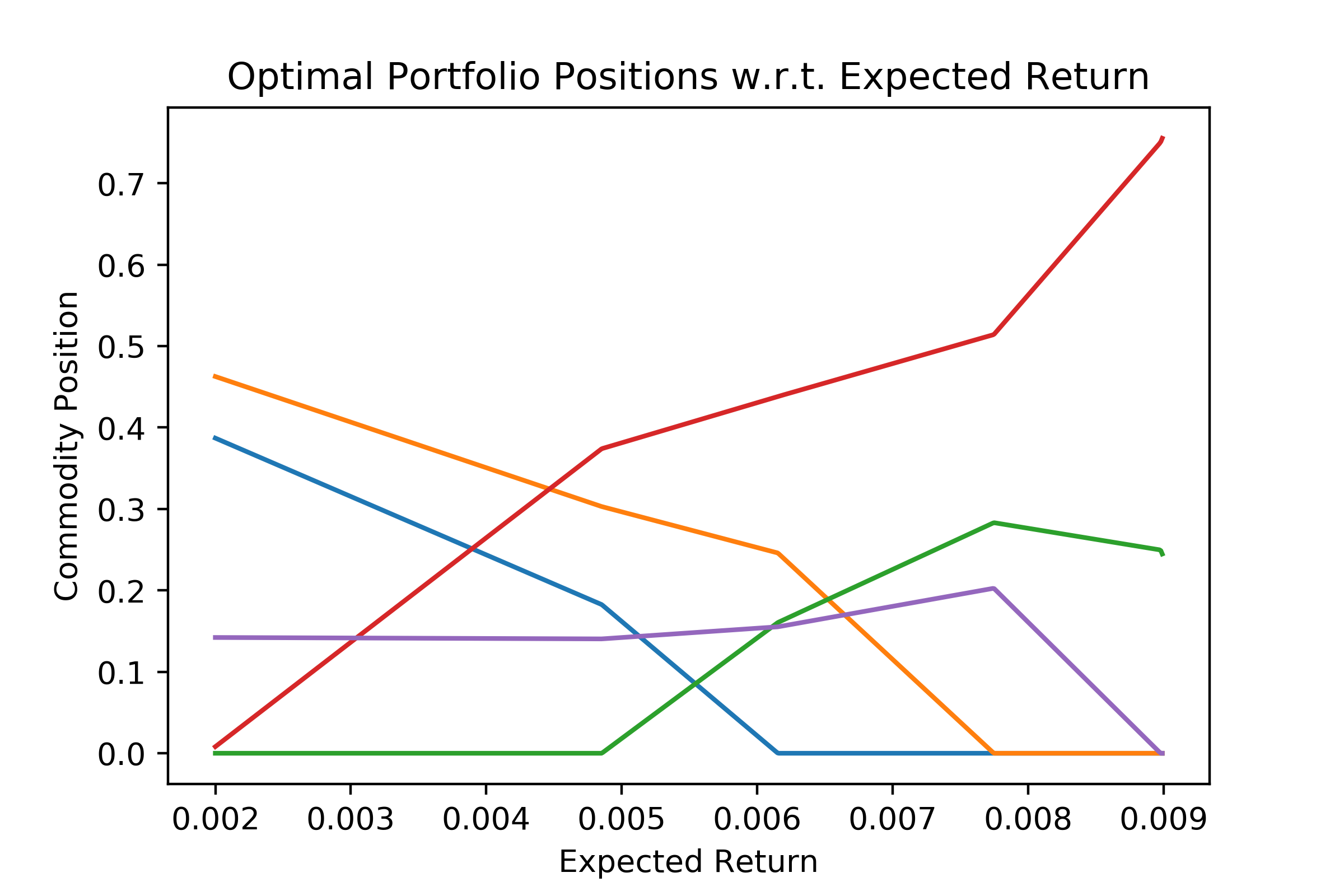
\[\begin{align*} z(\theta) = \min_{x} \frac{1}{2}\left[\begin{matrix}x_0\\x_1\\x_2\\x_3\\x_4\end{matrix}\right]^{T}\left[\begin{matrix}0.005515 & 0.0002831 & 0.006346 & 0.0005745 & -0.002589\\0.0002831 & 0.005018 & 0.002703 & -0.002481 & 0.00181\\0.006346 & 0.002703 & 0.009451 & -0.001497 & -0.002549\\0.0005745 & -0.002481 & -0.001497 & 0.005311 & -0.001545\\-0.002589 & 0.00181 & -0.002549 & -0.001545 & 0.01054\end{matrix}\right]\left[\begin{matrix}x_0\\x_1\\x_2\\x_3\\x_4\end{matrix}\right]&\\ \left[\begin{matrix}-1.0 & 0 & 0 & 0 & 0\\0 & -1.0 & 0 & 0 & 0\\0 & 0 & -1.0 & 0 & 0\\0 & 0 & 0 & -1.0 & 0\\0 & 0 & 0 & 0 & -1.0\end{matrix}\right]\left[\begin{matrix}x_{0}\\x_{1}\\x_{2}\\x_{3}\\x_{4}\end{matrix}\right]&\leq\left[\begin{matrix}0\\0\\0\\0\\0\end{matrix}\right]+\left[\begin{matrix}0\\0\\0\\0\\0\end{matrix}\right]\left[\begin{matrix}\theta_{0}\end{matrix}\right]\\ \left[\begin{matrix}0.002579 & 0.0007875 & 0.00711 & 0.009598 & 0.003935\\0.4472 & 0.4472 & 0.4472 & 0.4472 & 0.4472\end{matrix}\right]\left[\begin{matrix}x_{0}\\x_{1}\\x_{2}\\x_{3}\\x_{4}\end{matrix}\right]&=\left[\begin{matrix}0\\0.4472\end{matrix}\right]+\left[\begin{matrix}0.9999\\0\end{matrix}\right]\left[\begin{matrix}\theta_{0}\end{matrix}\right]\\ \left[\begin{matrix}-1.0\\1.0\end{matrix}\right]\left[\begin{matrix}\theta_{0}\end{matrix}\right]&\leq\left[\begin{matrix}0\\1.0\end{matrix}\right] \end{align*}\]We plug this into our favorite multiparametric solver (mine is the one I developed); this takes 12.1 ms in my solver (cough). We can now look at the optimal portfolio positions with respect to expected return. We see the classic piecewise affine behavior of parametric Quadratic Programs in this plot.

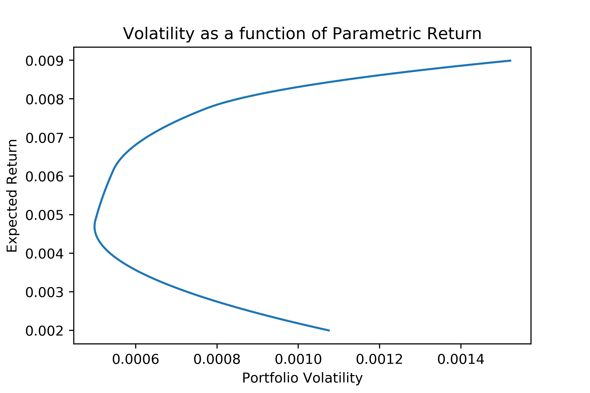
We successfully recovered the Pareto front! And see the entire range of possible expected returns with our assumptions (no negative positions, only one portfolio, etc.). Since all of the example images of what this should look like are not free use, I will direct you to compare this against expected Pareto fronts avalible on the internet. As a side note, this can be used by anyone for any purpose.
