This post returns to Hercules, the QUBO solver that has slowly taken over a fairly large number of posts on this blog. The last few times I wrote about this, the main story was that branch and bound is not magic, but if we give it better bounds, better problem reformulations, and a better preprocessor, then the number of subproblems can fall by a pretty large amount.
Since then, the solver has changed quite a bit. The change I want to focus on here is fairly high level, but it has a very real effect on solve time: the preprocessor is much stronger now due to using the roof dual to fix variables during the root and child node processing. The roof dual also gives a lower bound, but in this post I mostly want to focus on the variable-fixing side.
This is not going to be a detailed implementation post. There is quite a bit of machinery under the hood now, and a code walk through would probably be less useful than describing why the pieces fit together. So, the goal here is to sketch the new preprocessing path and then show how it changes both solve time and the size of the branch and bound tree.
The Problem, Again
As usual, we are looking at QUBO problems.
\[\begin{align} \min_{x\in\mathbb{B}^n} \frac{1}{2}x^TQx + c^Tx \end{align}\]The difficulty is not evaluating this function or even finding good solutions in many cases. The difficult part is proving that a good solution is actually the global optimum. This is why branch and bound is useful, but also why branch and bound can become painful. If the solver can fix variables, then we avoid creating many of those branches in the first place.
Branch and Bound (and its siblings) gives us two very different levers to pull to effect the algorithm.
- Domain reduction
- Stronger lower bounds
The newer versions of Hercules have gotten much better at both. We will be talking about the first one in this post.
Roof Dual Preprocessing
In an earlier post, I talked about persistency as a way to identify variables that must take a particular value in any optimal solution. The basic idea is that if we can prove one value of a variable cannot appear in any global optimum, then the variable must take the other value. That variable is fixed before we hand it to the subproblem solver, and we get to keep that variable fixed for all children nodes. The roof dual gives us a really easy way to generate these certificates.
Hammer’s description of the roof dual is a little more intuitive than most [2]. For the roof-dual discussion, it is convenient to rewrite the quadratic objective in edge-coefficient form.
\[\begin{align} f(x) = c_0 + \sum_i c_i x_i + \sum_{(i,j)\in E} c_{ij}x_ix_j, \end{align}\]split the edges by sign,
\[\begin{align} P &= \{(i,j)\in E : c_{ij} > 0\},\\ N &= \{(i,j)\in E : c_{ij} < 0\}. \end{align}\]For $\lambda_{ij}\in[0,1]$, define
\[\begin{align} \nu_0(\lambda) &= c_0 - \sum_{(i,j)\in P} c_{ij}\lambda_{ij},\\ \nu_i(\lambda) &= c_i + \sum_{\substack{j:(i,j)\in P}} c_{ij}\lambda_{ij} + \sum_{\substack{j:(j,i)\in P}} c_{ji}\lambda_{ji}\\ &\quad + \sum_{\substack{j:(i,j)\in N}} c_{ij}\lambda_{ij} + \sum_{\substack{j:(j,i)\in N}} c_{ji}(1-\lambda_{ji}). \end{align}\]Then the roof dual can be written as the LP
\[\begin{align} \max_{\lambda,\eta}\quad &\nu_0(\lambda) + \sum_i \eta_i\\ \text{s.t.}\quad &\eta_i \leq \nu_i(\lambda), \quad \forall i\\ &\eta_i \leq 0, \quad \forall i\\ &0 \leq \lambda_{ij} \leq 1, \quad \forall (i,j)\in E. \end{align}\]This is choosing the best linear lower bound induced by the quadratic terms. The value of that linear function at its own minimum is the certified lower bound.
It has a very nice extra property: when the roof dual solution labels a variable, that label is persistent. In plain terms, if the roof dual certifies $x_i=1$, then we can fix $x_i=1$. Similarly, if it certifies $x_i=0$, then we can fix $x_i=0$. If the roof dual leaves the variable unlabeled, then we leave it in the problem. [1]
\[\begin{align} \nu_i > 0 &\implies x_i = 0, \\ \nu_i < 0 &\implies x_i = 1, \\ \nu_i = 0 &\implies \text{no certified fixing.} \end{align}\]There are several equivalent ways to arrive to the bound generate above and the variable fixing machinery, in Hammer’s paper he shows us four. The local consistency LP relaxation of the pairwise binary problem gives the same roof-dual value, and so does the max-flow/min-cut construction discussed below. But Hammer’s LP is the one I find easiest to understand: rewrite the objective as a lower bound plus nonnegative leftovers. In the graph view, the labels are much easier to read: after the max-flow/min-cut solve, the residual graph tells us which literals are forced. That is the version Hercules actually uses. The LP is mainly useful here because it explains what lower bound is being optimized.
This is why the roof dual is so useful as a preprocessor. It is not just giving a lower bound; it is giving direct information about which variables can be removed from the branch and bound problem before the tree is even created. Even better, this pass can be iterated, and it can find new variables to provably fix.
This is a big deal because fixed variables compound. If we fix 10 variables, then in the worst possible enumeration view we cut away a factor of $2^{10}$ possible assignments. Of course, branch and bound is not doing raw enumeration, but still we want to use as much information as possible (that we can get cheaply). Every variable that is fixed at the root is one less variable that can split the tree later.
The other important part is that fixing variables changes the subproblems themselves. If $x_i$ is fixed to some value $p_i$, then that term can be substituted for that subproblem and any decendant subproblems. If $\mathcal{F}$ is the set of fixed variables and $\mathcal{R}$ is the remaining set, then for a symmetric QUBO we can write the reduced problem as follows.
\[\begin{align} \min_{x_{\mathcal{R}}\in\mathbb{B}^{|\mathcal{R}|}} \quad &\frac{1}{2}x_{\mathcal{R}}^TQ_{\mathcal{R}\mathcal{R}}x_{\mathcal{R}} + \left(c_{\mathcal{R}} + Q_{\mathcal{R}\mathcal{F}}p_{\mathcal{F}}\right)^Tx_{\mathcal{R}} + \text{constant} \end{align}\]This is one of those changes that sounds almost too simple once stated. If we already know the value of a variable, then stop carrying it around. However, in a branch and bound solver this matters quite a bit because every node solve gets cheaper, and each child problem gets smaller as more variables are fixed.
A somewhat important thing to point out is that this does not need to be solved by calling a LP solver. The same roof-dual bound can be obtained from an equivalent graph construction: build a graph on literals, solve a max-flow/min-cut problem, and read the persistent labels from the residual graph. In practice, this means we can solve it fairly quickly with an off the shelf graph package, which is what we do using petgraph. [1]
What the New Preprocessing Routines Buy Us
If we compare the old version of Hercules against the current version while still using QP subproblems, then we get a fairly clean view of what the roof dual and the new preprocessing path are buying us.
For this benchmark, the baseline is Hercules 0.5.0, and the current version is Hercules 0.6.3. These runs are based on the BQP100 problem instances from literature, and both use the same branching rule that is “branch on the variable that has the largest absolute value sum of coefficents”. Hercules 0.5.0 uses the old QP relaxation path with ClarabelQP, and Hercules 0.6.3 uses a box QP solver I wrote, HerculesABQP (available on crates.io, also has a python interface).
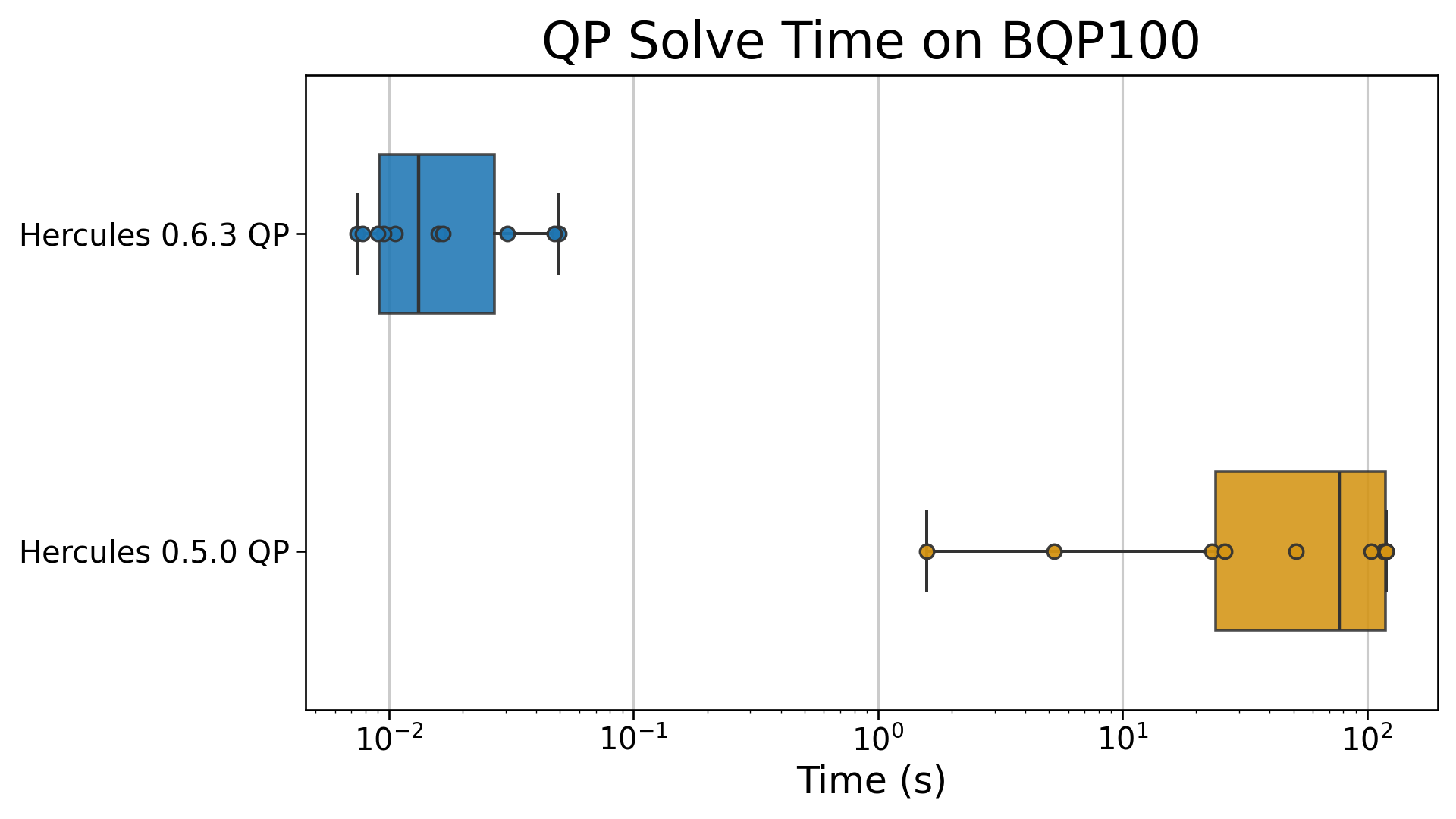
This is the part of the result that I find most interesting from a solver writing perspective. We are still using QP subproblems here, but the BQP100 median drops from 77.5 seconds to 0.0132 seconds, roughly a 5,800x speedup. That speedup is primarily the new version doing a much better job shrinking the problem, fixing variables, and avoiding a large branch and bound tree, along with a bunch of small memory allocation optimizations.
Solve time is useful, but it mixes together a few different things: preprocessing speed, subproblem solver speed, and the actual shape of the branch and bound tree. To see whether Hercules is really doing a better job shrinking the search, it helps to look directly at the number of nodes visited.
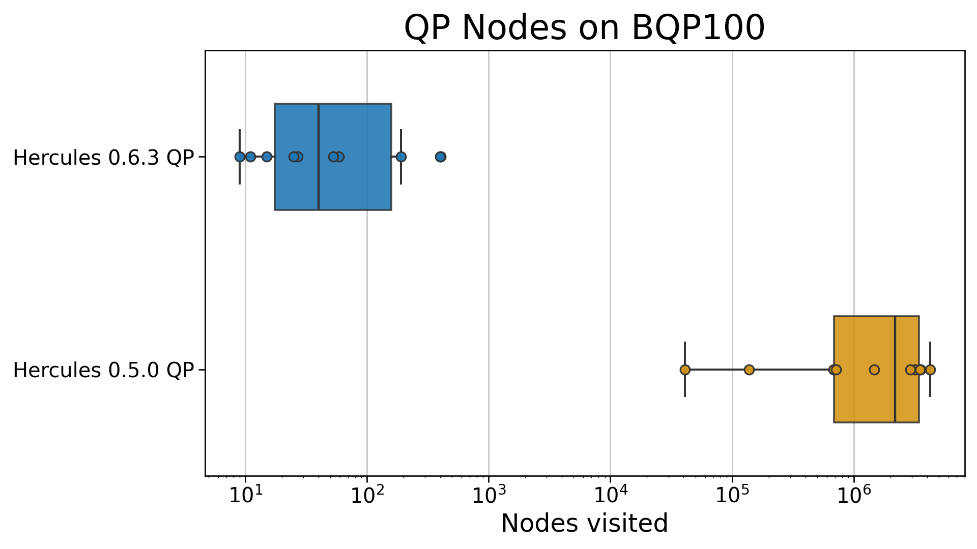
This is a much better way to see the effect of the new preprocessing path. On BQP100, the median number of visited nodes drops from about 2.19 million in Hercules 0.5.0 QP to 40 in Hercules 0.6.3 QP. That is a reduction of over 50,000x. The node counts suggest that the roof dual variable fixer is doing its job.
Wrapping Up
The overall story is that Hercules is becoming less of a naive branch and bound solver with a few helpers bolted on, and more of a modern branch and bound implimentation. The roof dual helps remove variables from the problem before they are allowed to become branches. The QP solver is still in the loop, but it is now being handed much smaller problems and many fewer nodes.
The next step is using the MixingCut SDP relaxation solver as the main relaxation problem solver inside Hercules, but that is a separate story. Also at some point, I will need to deal with problem symmetry in an inteligent way.
Citation
[1] - Boros, E., Hammer, P. L., Sun, R., & Tavares, G. (2008). A max-flow approach to improved lower bounds for quadratic unconstrained binary optimization (QUBO). Discrete Optimization, 5(2), 501-529.
[2] - Hammer, P. L., Hansen, P., & Simeone, B. (1984). Roof duality, complementation and persistency in quadratic 0-1 optimization. Mathematical Programming, 28(2), 121-155.