In today’s post, I will talk about a particular form of square matrices that Tridiaginal Matrices. These are matrices where the only nonzero elements are on the main diagonal and the diagonals directly above and below the main diagonal. These matrices can be visualized in the example below, where A is a tridiagonal matrix. Matrices of this type show up in science and engineering computations quite often, and these matrices have specialized algorithms to solve linear systems based on tridiagonal systems. The speedup can be quite dramatic, switching from a general linear systems solver to specialized tridiagonal solvers.
\[A = \begin{pmatrix} 5 & 2 & 0 & 0 & 0\\ 1 & 3 & 4 & 0 & 0\\ 0 & 1 & 3 & 2 & 0\\ 0 & 0 & 2 & 7 & 1\\ 0 & 0 & 0 & 3 & 10 \end{pmatrix}\]From the perspective of a linear system, $Ax = f$. What this is saying in practice is that we have $n$ equations of the following form. Where $a,b,c$ are the row below the main diagonal, the main diagonal, and the diagonal above the main diagonal (have I said diagonal enough times?). As a matter of convention we have made $a,b,c$ vectors of the same length and $a_1 = 0, c_n = 0$.
\[a_ix_{i-1} + b_ix_i + c_ix_{i+1} = f_i\]A situation where this sort of equation set can arise when trying to solve a Poisson equation in 1 dimension. We are trying to solve for $u(x)$. The Poisson equation can be discretized via central finite differences.
\[\nabla^2 u = f \rightarrow \frac{d^2}{dx^2}u(x) = f(x)\quad (1)\] \[\frac{d^2}{dx^2}u(x_i) \approx \quad \frac{u(x_{i+1}) - 2u(x_i) + u(x_{i-1})}{h^2} \quad (2)\] \[u(x_{i+1}) - 2u(x_i) + u(x_{i-1}) = h^2 f(x_i) \quad (3)\]So we can create a linear system of equations in terms of $u_i = u(x_i)$ to solve this differential equation. This particular equation pops up a lot in scientific computing, so it is essential to use specialized algorithms to deal with these problems. Otherwise, there is a strong chance that it would otherwise be computationally infeasible.
Thomas elimination is a specialized algorithm to solve systems of this type. Since we know beforehand that this matrix is tridiagonal, we can exploit this. Thomas elimination algorithm In asymptotic terms, Thomas elimination, and its derivatives are $\mathcal{O}(n)$ scaling algorithms. In contrast, Gaussian elimination is $\mathcal{O}(n^3)$ scaling, where $n$ is the number of variables in the linear system.
The algorithm is a two-step process, eliminating the $a$ diagonal and then solving the bidiagonal system with back substitution.
The first step is creating new $c$ and $f$ vectors by the following method.
\[c'_i = \begin{cases} \frac{c_i}{b_i} & i = 1\\ \frac{c_i}{b_i - a_i c'_{i-1}} & i = 2,\dots, n-1\\ \end{cases}\] \[d'_i = \begin{cases} \frac{d_i}{b_i} & i = 1\\ \frac{d_i - a_i d'_{i-1}}{b_i - a_i c'_{i-1}} & i = 2,\dots, n\\ \end{cases}\]Then the second step, back substitution, we have
\(x_n = d'_n\) \(x_i = d'_{i} - c'_i x_{i+1}, i = n-1, \dots, 1\)
I have implemented this in Python 3.7 with NumPy. Of course, there are much faster public implementations that can be found in the scipy.linalg package. This is just an example implementation.
import numpy

def thomas_elimination(a, b, c, d):

    c_prime, d_prime = c.copy(), d.copy()
    n = a.shape[0]
    x = numpy.zeros(n)
    #handle the i = 0 initial case
    c_prime[0] = c[0]/b[0]
    d_prime[0] = d[0]/b[0]

    #forward elimination
    for i in range(1,n):
        denominator = b[i] - a[i]*c_prime[i-1]

        c_prime[i] = c[i]/denominator
        d_prime[i] = (d[i] - a[i]*d_prime[i-1])/denominator

    #back propigation
    x[n-1] = d_prime[n-1]

    for i in range(n-2, -1, -1):
        x[i] = d_prime[i] - c_prime[i]*x[i+1]

    return x
Now that we have some example code, let’s try to solve the motivating problem. Here we will discretize the following Poisson boundary value problem and solve it via the Thomas Elimination algorithm.
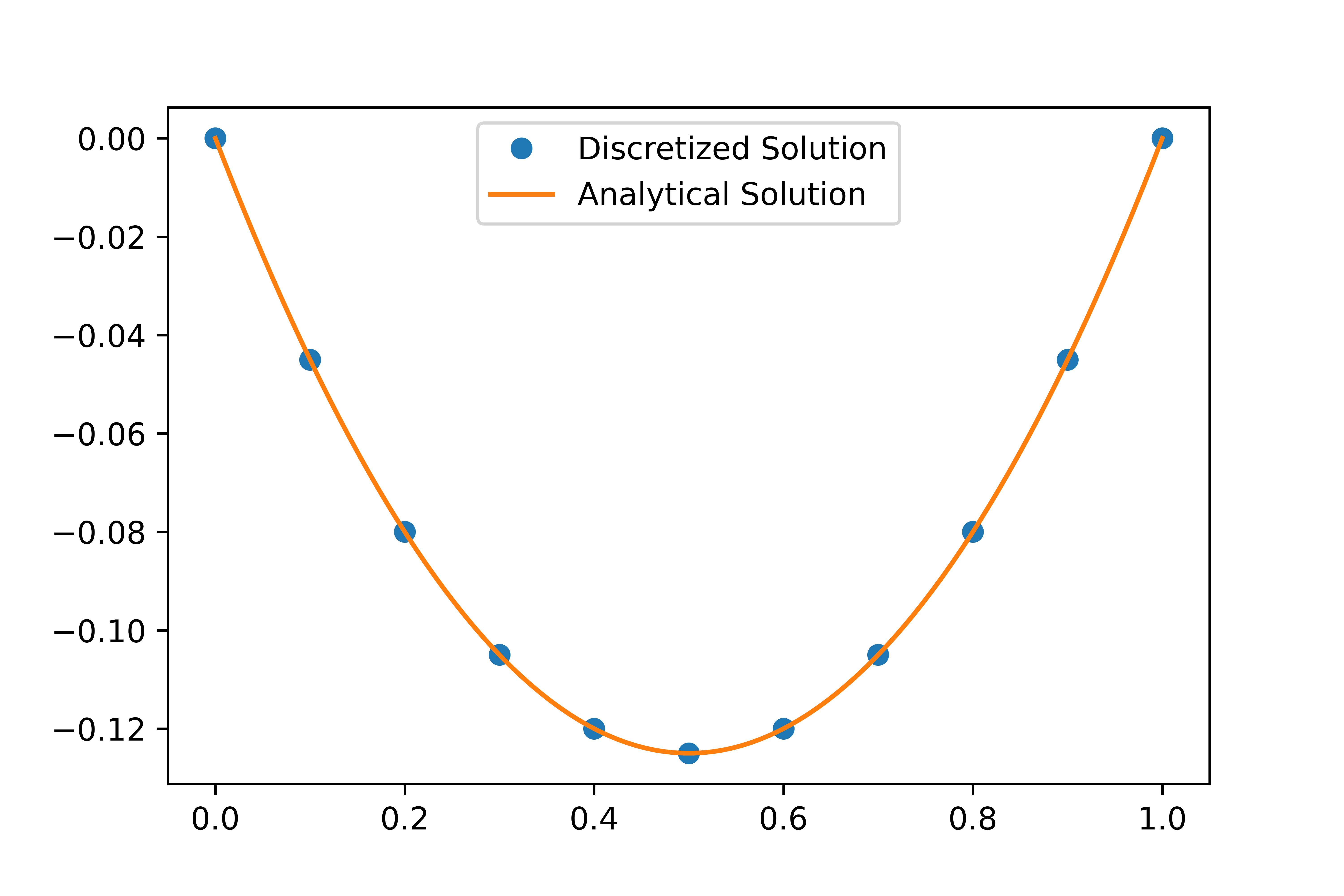
\[\frac{d^2}{dx^2}u(x) = 1, u(0) = u(1) = 0\] \[u_0 = 0\] \[u_{i-1} - 2u_i + u_{i+1} = h^2\] \[u_n = 0\]We have the values of $a,b,c,d$, and we can feed this into the faster algorithm! Here is the discretized solution vs. the analytical answer.

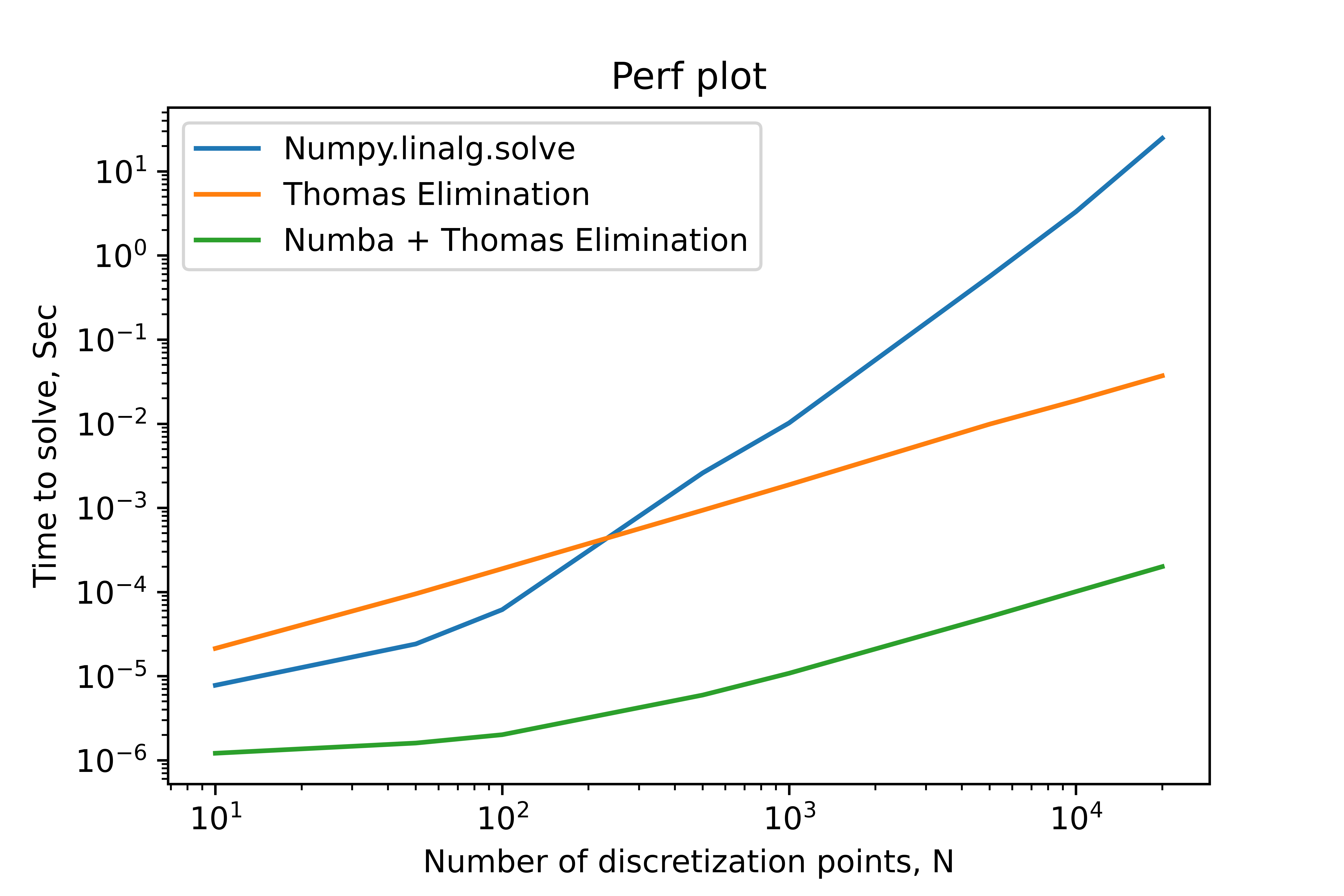
We are looking at the time it takes to solve with a different number of discretization points, $N$. This benchmark does not include any setup work and only includes the time to solve the linear system. As we can see in the plot below, this is multiple orders of magnitude faster than the naive gaussian procedure. If we use the numba package to compile the algorithm, we get another two orders of magnitude improvement.
