Applications of Optimization - Ridge Regression

Ridge regression is a variation of least squares in that it adds a penalty to having large parameter values. This penalty is tunable and will change the model bias-variance trade-off. For a linear unconstrained ridge regression, the objective takes the following form: both norms are taken in the l2 sense.

This has the following gradient.

We can solve this optimization problem rather simply since $f$ is convex, by setting the gradient equal to zero and solving the resulting equation.

If you specify a nonzero $\lambda$, this system is always invertible; therefore, we always have a unique solution. Modern BLAS packages can solve this linear system quite efficiently. But in general, solving linear systems has a time complexity of $\mathcal{O}(n^3)$ where n is the dimensionality of the number of parameters. For systems of less than a few thousand examples, however, this is not a difficult task. Since we have an expression for the gradient, we can also employ a host of interactive unconstrained optimization methods without numerical approximation to tackle this problem, such as gradient descent and conjugate gradient methods. I will not be writing the code for that here, but I will compare various gradient descent algorithms using this as a test problem in a future post.

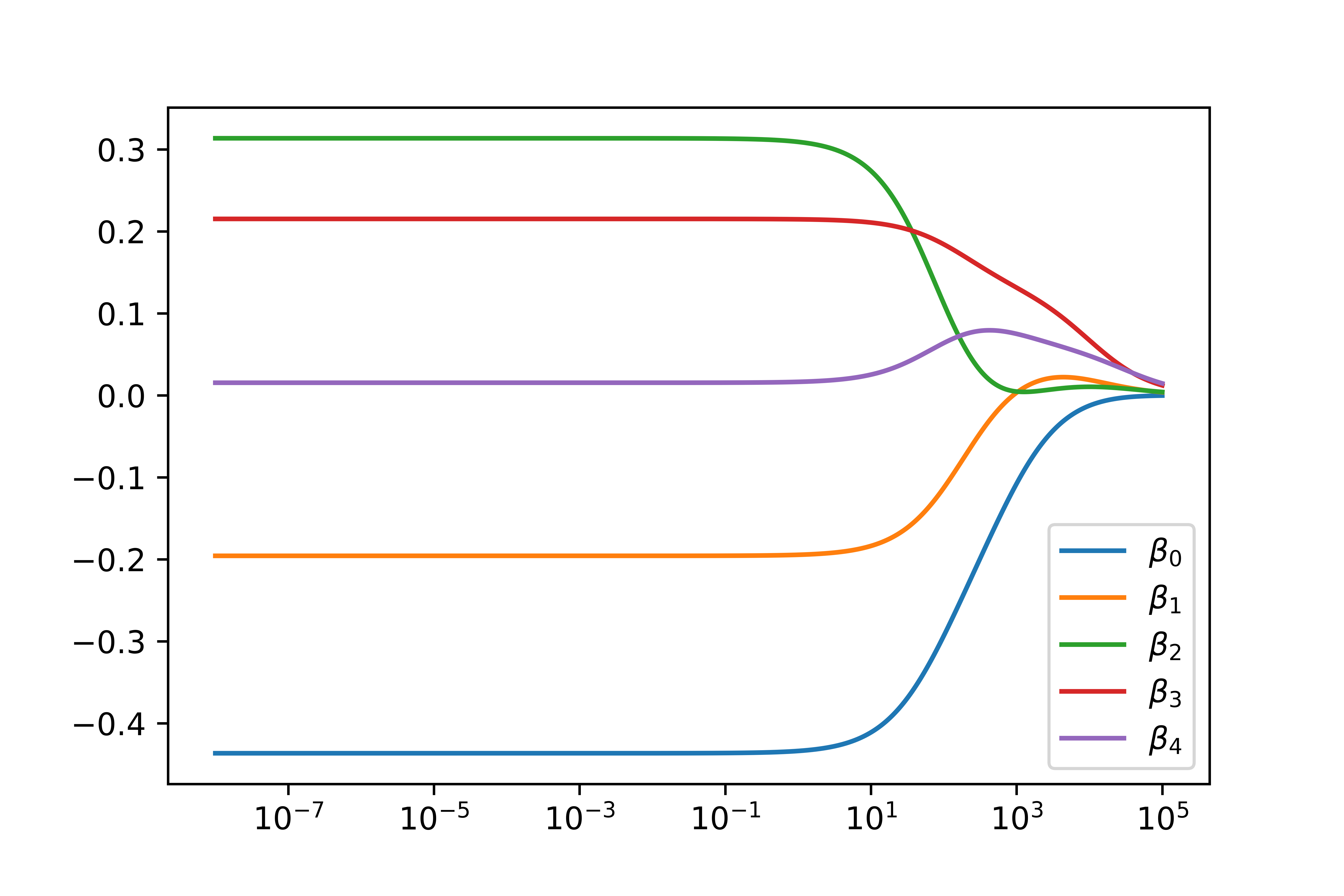
Here I will compute the ridge plot of a noisy model generated from a 4th order polynomial to show how the $\lambda$ parameters have on the regressed parameters. I included all of the python 3.7 code required to generate these plots at the bottom.

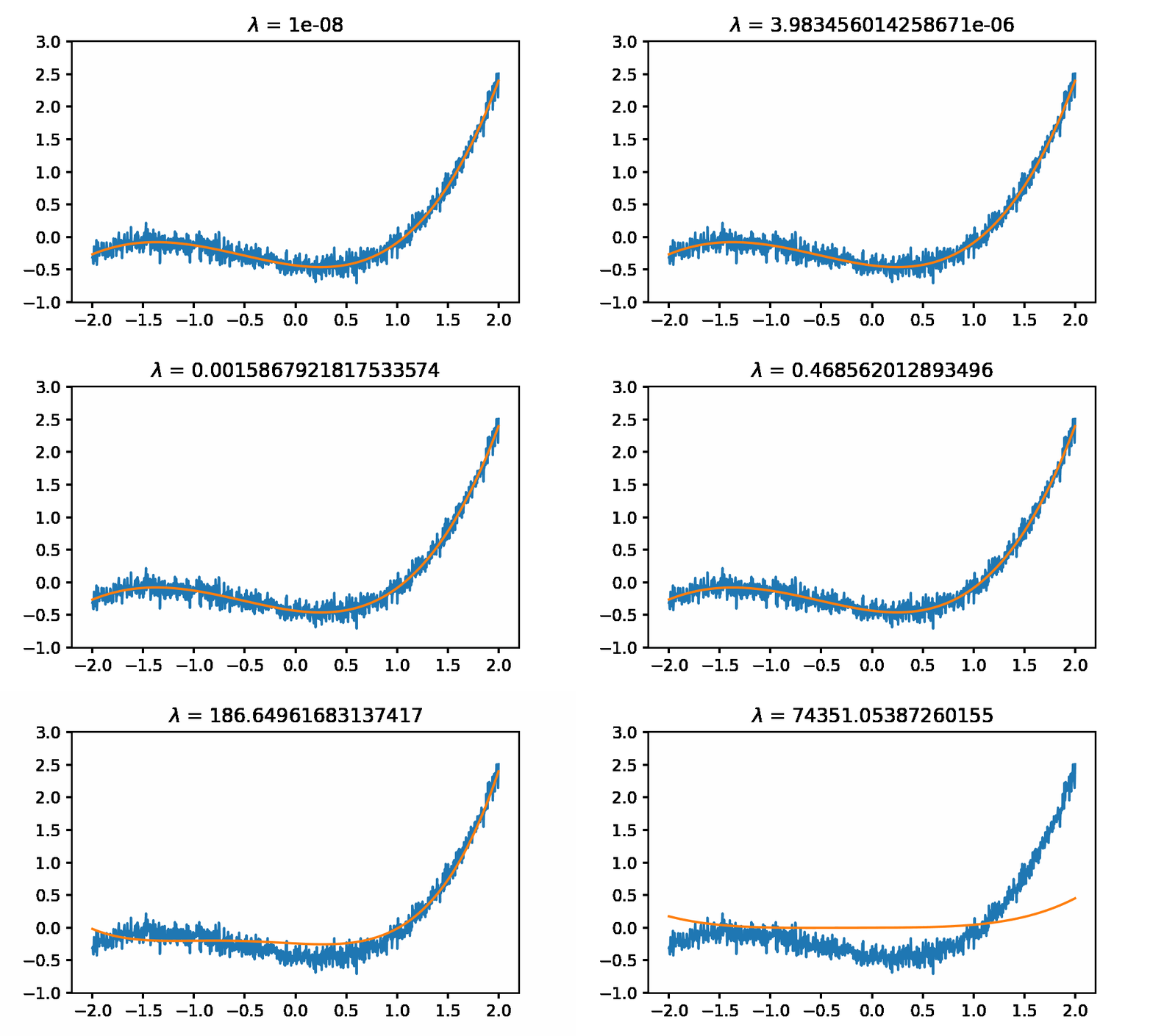
And this is what the regressed functions look like as you change the $\lambda$ parameter.

#generate random polynomial coefficents
cooef = numpy.random.rand(5) - .5
#generate 1000 evenly spaced points between 0 and 2
p = numpy.linspace(-2, 2, 1000)

#Build our A matrix
A = numpy.block([[0*p+1], [p], [p**2], [p**3], [p**4]]).T

# generate our data points
y = A@cooef + .1*numpy.random.randn(1000)

#solve the ridge regression over lambda [10^-5, 10^3] spaced exponentially 

lambdas = numpy.power(10, numpy.linspace(-8, 5, 10000))

#pre-cache some common veriables
b = A.T@y
P = A.T@A
regressed_cooefs = numpy.zeros((10000, 5))

for i, lambda_ in enumerate(lambdas):
    regressed_cooefs[i] = numpy.linalg.solve(P + lambda_*numpy.eye(P.shape[0]), b)

plt.plot(lambdas, regressed_cooefs)
plt.xscale('log')
plt.legend( [rf'$\beta_{i}$' for i in range(5)])

And here is the code to generate the gif

import gif

@gif.frame
def plot_step(i:int):
    fig, ax = plt.subplots(figsize=(5,3), dpi = 200)
    ax.plot(p, y)
    ax.plot(p, A@regressed_cooefs[i])
    ax.set_title(rf'$\lambda$ = {lambdas[i]}')
    ax.set_ylim((-1, 3))
frames = []

for i in range(len(lambdas)):
    if i % 100 == 0:
        frame = plot_step(i)
        frames.append(frame)

gif.save(frames, 'yehaw.gif', duration=5, unit='s', between='startend')