The optimal approximation is finding an approximate function that minimizes some objective function based on the difference between your original and approximate function. This can be stated as a min-max problem. This post will look at the following optimization problem: we are looking for the $n^{th}$ order polynomial that minimizes the maximum error. This is typically called the ‘best polynomial approximation,’ but what is optimal depends entirely on what your objective function is.
\[\min_{P\in\mathcal{P}^n} \max_{-1\leq x\leq 1} |F(x) - P(x)|\]The applications of this are far-reaching; almost every time a computer calculates a higher-order function, such as a Trig or a Bessel function, it is almost always evaluating a ‘best approximation.’ As a side note, this is not the only form that a best approximate can take; rational approximation is another important topic in the field.
The typical algorithm used to solve these problems is the Remez Algorithm. The algorithm is a relatively simple iteration scheme composing of three parts. Given a function $F$ and polynomial order $n$, we have the following scheme.
-
Solve the following linear system, $b_0 + b_1x_i + \dots + b_nx_i^n + (-1)^iE = F(x_i), i\in{1,\dots,n+2}$, where $x_i$ is in your set of points $K$.
-
Used the solved coefficents ${b_i}$ to create the residual function $F(x) - P(x)$
-
Reset $K$ to the local extreme points of the residual function.
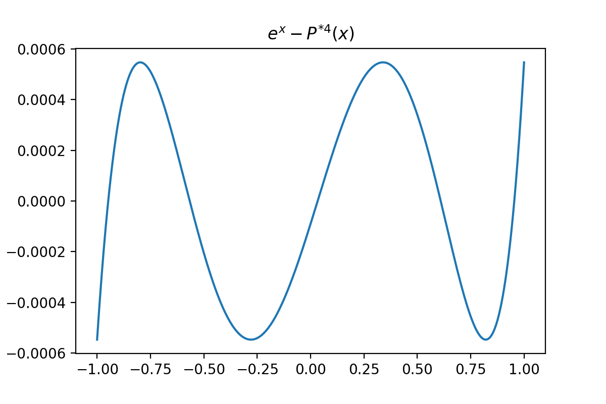
The theoretical basis for this algorithm is from the Equioscillation theorem , that effectively states if $P$ is the optimum then there must be $n+2$ points of alternating sign where $abs(F(x_i) - P(x_i)) = abs(F(x_j) - P(x_j))$. The following plot is the error, $F(x) - P(x)$, of the best $4^{th}$ order polynomial approximation of $e^x$. Here we can see that the largest values are attained 6 times and of equal magnitude. This is where intuition on the $E$ term in the above algorithm comes, in, otherwise this algorithm has the appearance of ordinary least squares.

Now that we have the justifications out of the way, how do we actually do this?
We should start with step 0, the hidden step in this algorithm. We need an initial set of points, $K$. This should be taken as the Chebyshev nodes of order $n+2$ scaled to the region you need them in. Chebyshev nodes are the extrema of Chebyshev polynomials. You can think of this step as hot starting the algorithm with a good initial guess (which is usually a very good approximate).
Now that is out of the way; we can head to step 1. This is just setting up the system properly. This can be carried out with the following python code. The solution to the equation is the coefficients of the polynomial and the error term $E$. We want to split the error term away from the polynomial coefficients, which is done with the coeff variable.
# create an empty matrix and vector to hold the system
A = numpy.zeroes((n_degree+2, n_degree+2))
b = numpy.zeros(n_degree+2)

# fill the columns
for i in range(n_degree+1):
  A[:,i] = x_points**i
  b[i] = func(x_points[i])

# put in the last value
b[-1] = func(x_points[-1])

# add in the 'occilation condition'
E_array = numpy.array([(-1)**(i+1) for i in range(n_degree+2)])
A[:, n_degree+1] = E_array

params = numpy.linalg.solve(A, b)
coeffs = numpy.flip(params[:-1])
The second step is creating the residual function $F(x) - P(x)$. This is simple with a lambda.
r_i = lambda x: func(x) - numpy.polyval(coeffs, x)
The most complicated part of this process is step number 3, where we are trying to find our function’s local extrema. This is itself a two-part process. In the first part, we must bracket the extrema. Since we know that our points ${x_i}$ are on alternating signs of our residual, then we know that there must be a point between them were our residual is equal to $0$. So we use root-finding to do so. Since I am not using any derivative information, I did a bisection seach to find the zeros, but much more sophisticated methods exist such as Brent’s method.
def bisection_search(f, low, high):

    #flip high and low if out of order
    if f(high) < f(low):
        low, high = high, low

    #find mid point
    mid = .5*(low + high)

    while True:

        #bracket up
        if f(mid) < 0:
            low = mid
        #braket down
        else:
            high = mid

        #update mid point
        mid = .5*(high + low)

        #break if condition met
        if abs(high - low) < 10**-15:
            break

    return mid
Now that the extrema have been bracketed by a low and a high value, we can then find the extreme points. This is done with a central difference approximation to the derivative (since we still do not know what the derivatives are) and then bracketing the derivatives with the above bisection search.
def concave_max(f, low, high):
    #create an approximate derivative expression
    scale = abs(high - low)
    h = 10**(-5)*scale
    df = lambda x: (f(x + h) - f(x-h)) / (2.0*h)

    return bisection_search(df, low, high)
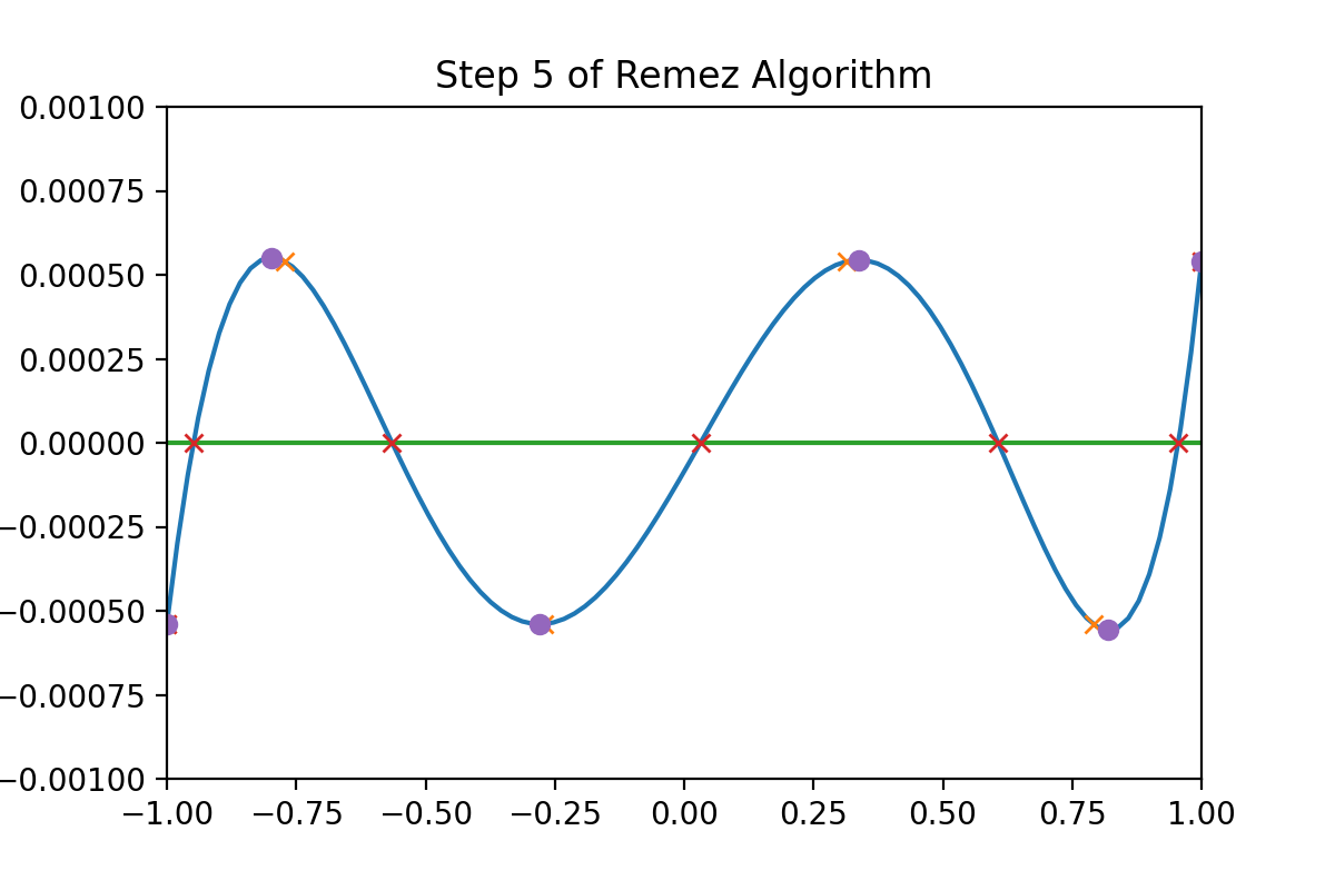
This gives us the extrema of the residual function. We update our points $K$ and then start back to step 1 if we do not terminate. An example of each step of this process can be seen below. The orange crosses are the initial points in $K$, the blue function is the residual, the red crosses are the brackets for the extrema, and the purple dots are the new extrema that we will use as $K$ for our next step.

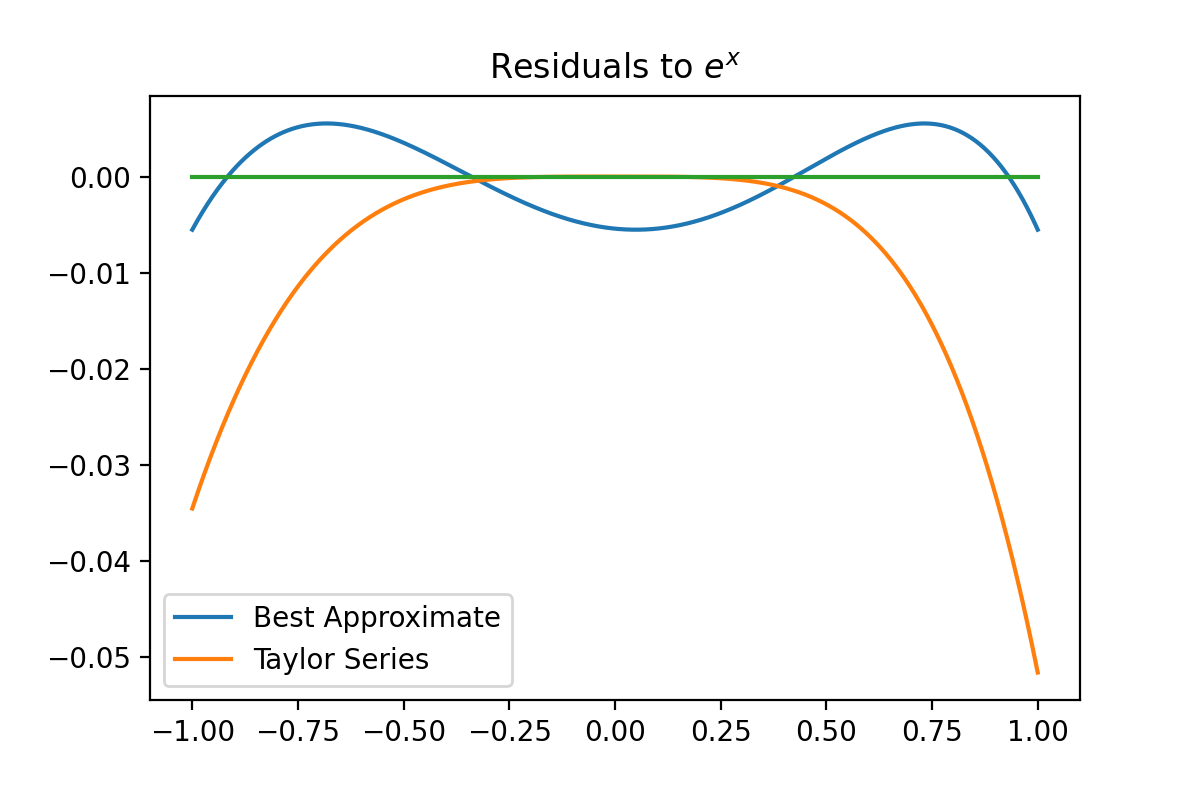
The python code that implements the Remez algorithm will be posted below (the extrema at the endpoints are not being calculated properly, I made a simplifying assumption that is not necessarily true. You have been warned). Here I want to compare the $3^{rd}$ order best polynomial and a Taylor series of equal order centered at 0. We can see that the Taylor series is much more accurate in the neighborhood of 0 but is an order worse near the edges. This is contrasted with the best approximate’s much more uniform error behavior. Most of the time, you would want to the behavior of the ‘best’ approximate, but not necessarily all of the time.

Here is the code dump. This can be modified to approximate functions over ranges other than $[-1,1]$ by scaling the initial points into that region.
def remez(func, n_degree):

    #initialize the node points

    x_points = chev_points(n_degree+2)
    max_iter = 100

    A = numpy.zeros((n_degree+2, n_degree+2))
    b = numpy.zeros(n_degree+2)
    coeffs = numpy.zeros(n_degree+2)

    #place in the E column

    E_array = numpy.array([(-1)**(i+1) for i in range(n_degree+2)])
    A[:, n_degree+1] = E_array

    for i in range(max_iter):

        #build the system

        for i in range(n_degree+1):
            A[:,i] = x_points**i
            b[i] = func(x_points[i])

        b[-1] = func(x_points[-1])

        #solve the system for polynomial coefficents
        params = numpy.linalg.solve(A, b)
        coeffs = numpy.flip(params[:-1])

        #build the residual expression
        r_i = lambda x: func(x) - numpy.polyval(coeffs, x)

        #create the intervals to bracket
        interval_list = [[x_points[i], x_points[i+1]] for i in range(len(x_points)-1)]

        intervals = [1]
        intervals.extend([bisection_search(r_i, *i) for i in interval_list])
        intervals.append(-1)

        #now that we have the brakets for the extermem
        extermum_interval = [[intervals[i], intervals[i+1]] for i in range(len(intervals)-1)]

        # solve for the extermum
        extremums = [concave_max(r_i, *i) for i in extermum_interval]

        # HEAVY ASSUMPTION
        extremums[0] = 1
        extremums[-1] = -1

        #update our set K
        x_points = numpy.array(extremums)

        # Termination criteria
        errors = numpy.array([abs(r_i(i)) for i in extremums])
        mean_errors = numpy.mean(errors)

        if numpy.max(numpy.abs(errors - mean_errors)) < 10**(-4)*numpy.max(errors):
            break


    return coeffs