Matrix Gradient Decent for Aggressive Controllers

I have been looking at matrix completion problems and other matrix-based minimization problems for a control application recently, where we are trying to determine a gain matrix $K$ that relates the current state, $x_t$, to the input action, $u_t$, that would stabilize the system and drive the system to the origin. This means by tuning the gain matrix, $K$, we can change how the system propagates with time. As we see below, we can typically design $A-BK$ to rapidly shrink as it is multiplied repeatedly. In this post, we will discuss how to find $K$, given that we want to make a very aggressive controller and not consider any objective (such as found by solving the DARE/CARE equations [1]).

\[\begin{align} x_{t+1} &= Ax_t + Bu_t\\ u_t &= -Kx_t\\ x_{t+1} &= (A-BK)x_t\\ x_{t+N} &= (A-BK)^Nx_t \end{align}\]

Which brings us to the problem we are trying to solve. We want to design the $K$ matrix to minimize the norm of $(A-BK)^2$, and while the gradient does have a close form, it is a nonlinear function of $K$. This means it might be rough to try to get a closed-form expression, so instead, we will use gradient descent to solve. Not only can use use gradent decent to find scalars and vectors but also matrices, which is quite cool!

\[\min_{K} f(K) = ||(A - BK)^2||_F\]

Gradient descent for this problem can be generally described by the following equation, which looks just like the normal equations for gradient decent, except that instead of using the gradient, we are utilizing the matrix derivative as our improvement direction [2]. On top of this, we select our step size parameter, $\gamma$, via an approximate line search, e.g., we have a set of trial step sizes, and we just simply pick the stepsize that minimizes the function value, denoted as $\gamma^*$ [3]. This should be iterated until adequate convergence is achieved or it is no longer decreasing.

\[K_{n+1} = K_{n} - \gamma^* \frac{\partial}{\partial K}f(K)\]

With that boilerplate out of the way, we can apply the gradient descent algorithm to the matrix problem. With a dynamic system described by the following $A$ and $B$ matrices, we want to find a $K$ such then we rapidly push the states to the origin.

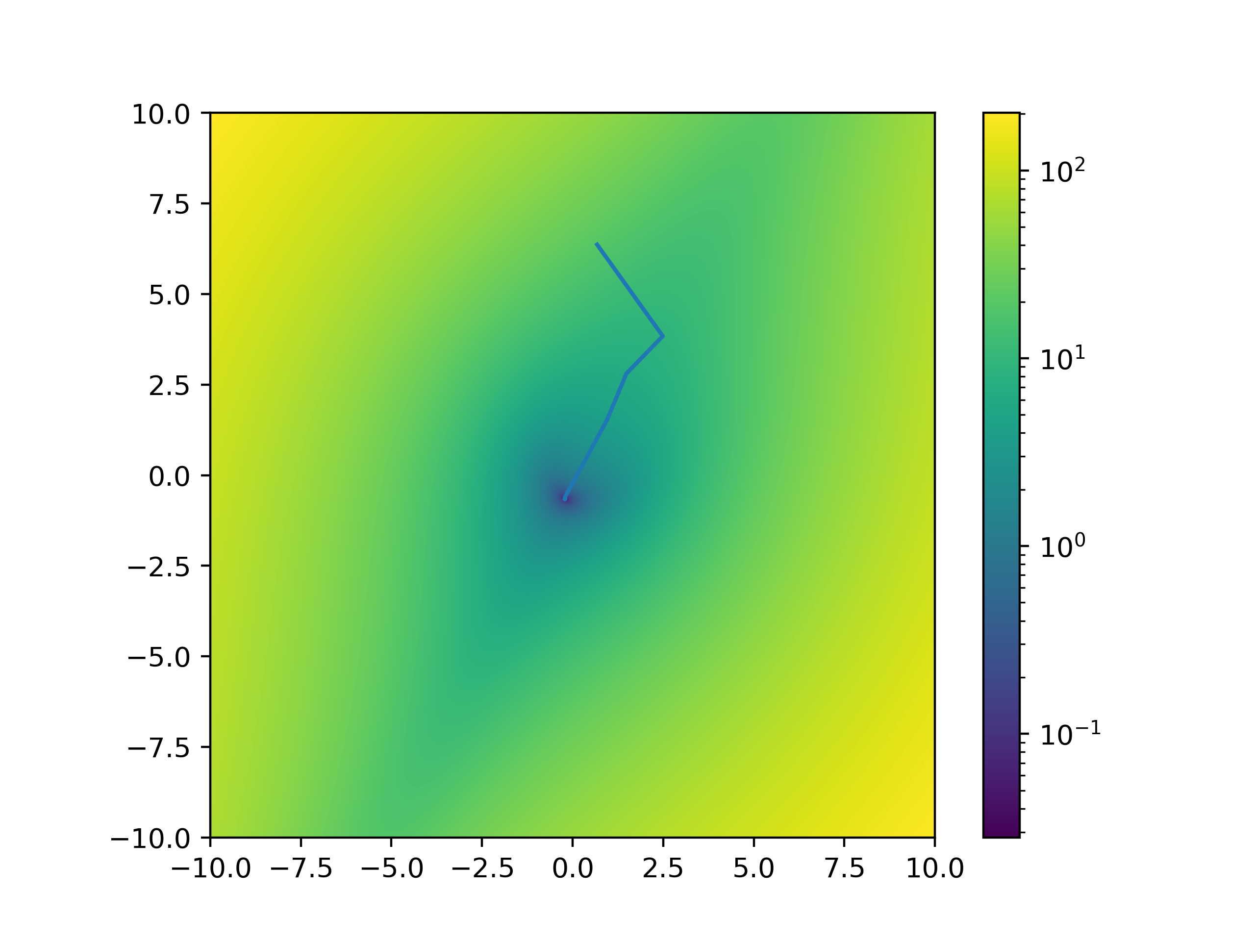
\[\begin{align} A = \begin{bmatrix} 0.18497671 & 1.01432116\\ -0.8661342 & -0.32058265 \end{bmatrix}&, \quad B = \begin{bmatrix} -0.48418357\\ -0.90051931 \end{bmatrix}\\ \end{align}\]

To start off with, we make a random guess of $K$. As $K$ is a matrix of two elements, $K_{0,0}$ and $K_{0,1}$, we can plot it against the function value. It starts from a high value and slides into the solution as we iterate.

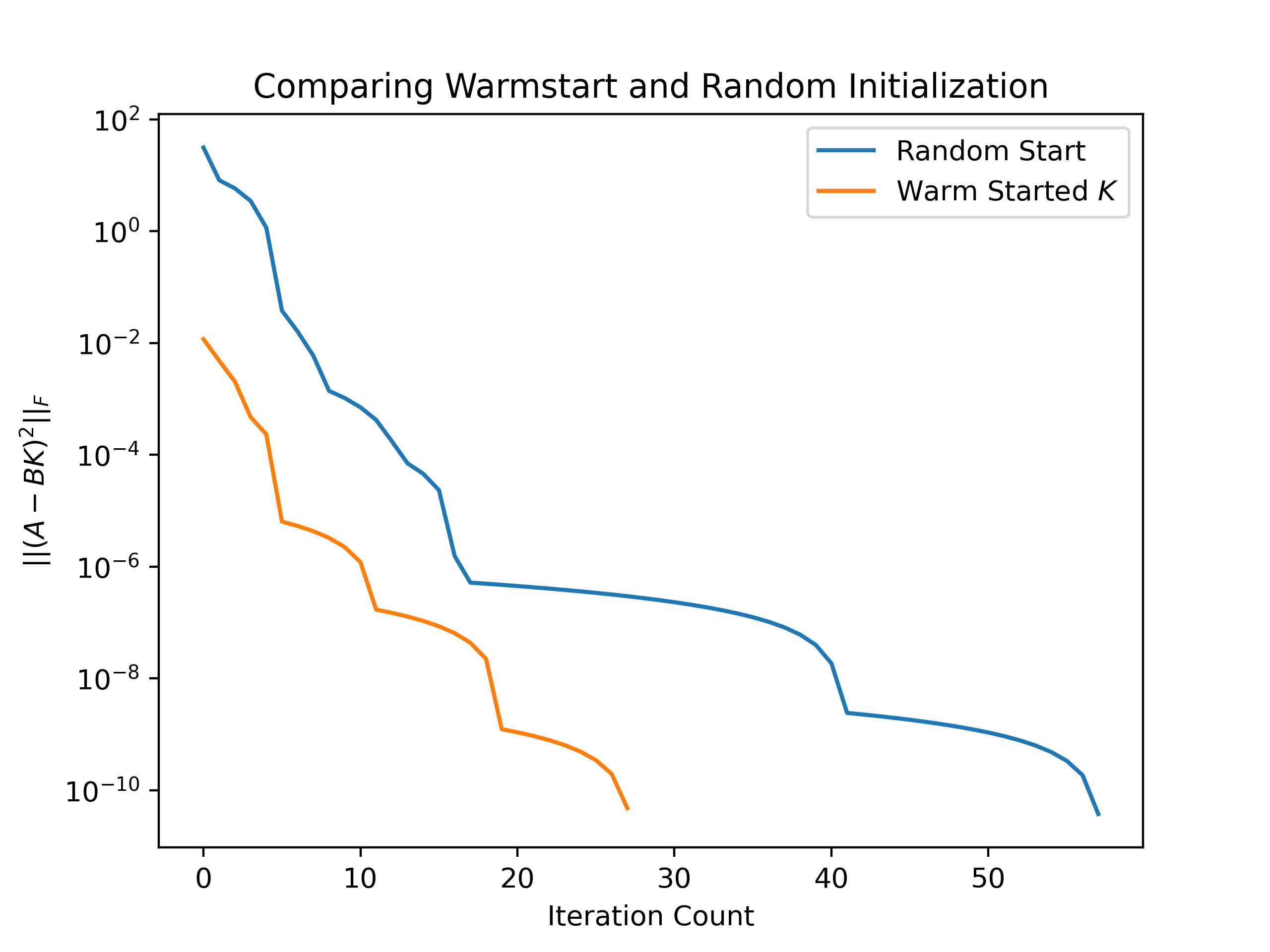
Now, it has been said that the speed of gradient descent is often a function of the initial guess, e.g., $K_0$; here, we can compare the progress of gradient descent with a better guess. Here, our better guess is the solution to $\vert\vert A - BK\vert\vert_F$, which is the least squares solution $K_0 = (B^TB)^{-1}B^TA$. This initial guess is quite a good guess for this problem as what minimizes $\vert\vert A - BK\vert\vert_F$, will probably do a good job at minimizing $\vert\vert(A - BK)^2\vert\vert_F$. We can see that compared to random initialization; this leads to a large reduction in the number of iterations and a much lower initial starting value.

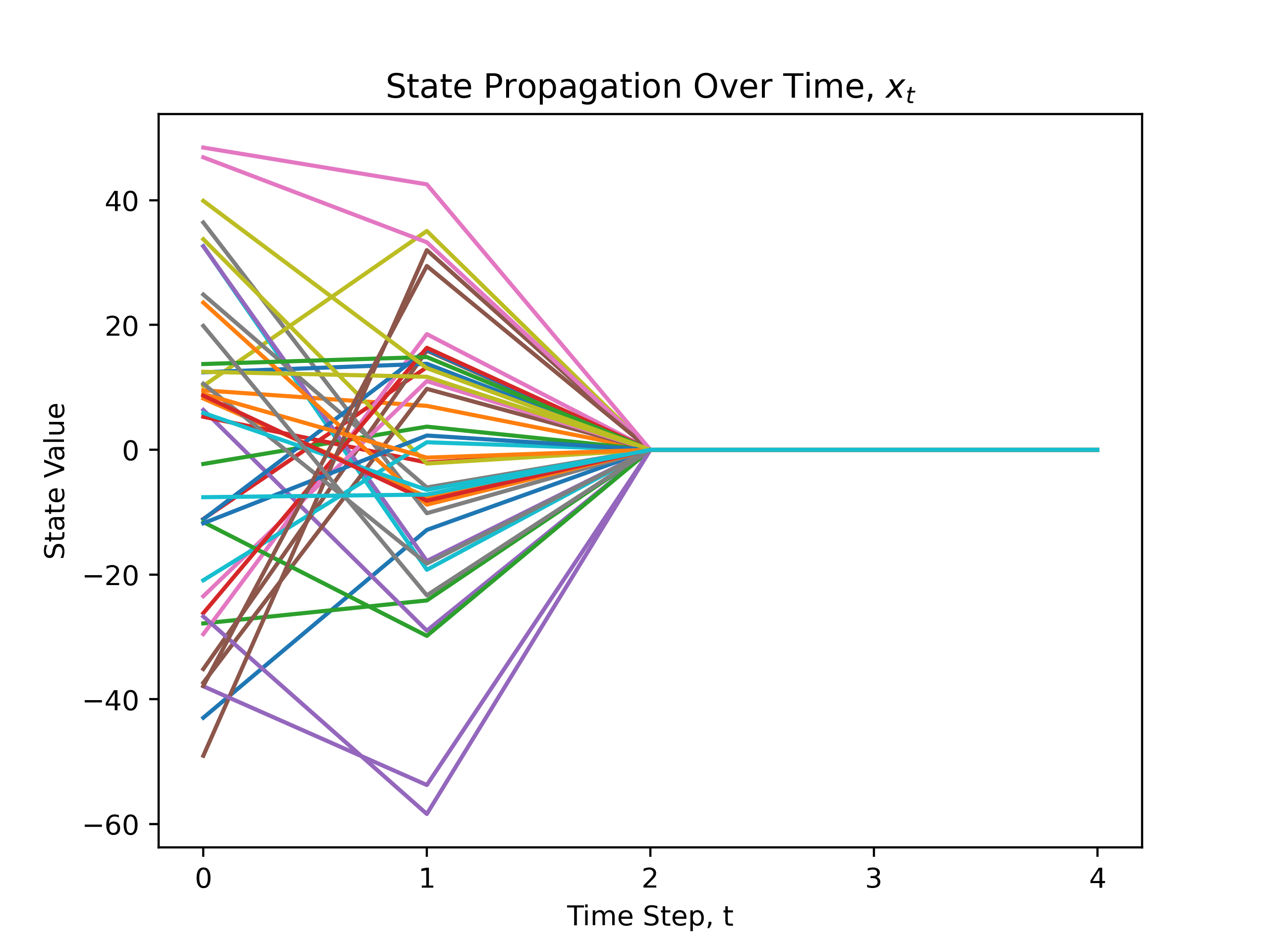
Returning to our initial problem, we can use this gain matrix to check if we have stabilized our system for different initial states. In this case, this generates a very aggressive controller, in that by the second time step $x_{2}$ in the absence of noise, we are within numerical error of the origin. Below, we have 30 random initial states of this system, and we see how it propagates with time of the gain matrix $K$, from gradient descent.

As always, a code sample for the gradient descent used here is provided, along with the gradient and value function of the problem.

def K_gradient_decent(A, B, K_0, max_iter:int = 1000):
    
    # some initial housekeeping 
    K = K_0
    cost = []
    
    # set of allowed steps
    steps = 10**numpy.geomspace(-.1, -10, 20)

    for i in range(max_iter):
        
        # calculate gradient and function value
        d_f = calc_gradient(A, B, K)
        current_cost = calc_function(A, B, K)
        
        # add current cost
        cost.append(current_cost)
        
        # find all possible new Ks give step sizes
        K_steps = [K - step*d_f for step in steps]
        
        # find the function values assosiated with these steps
        step_costs = numpy.array([calc_function(A, B, K_i) for K_i in K_steps])
        
        # find the best step index that minimizes the function value
        min_step_index = numpy.argmin(step_costs)
        
        # if we are still decreasing update K else break out
        if step_costs[min_step_index] <= cost[-1]:
            K = K_steps[min_step_index]
        else:
            break
    
    return K, cost

def calc_gradient(A, B, K):
    T_0 = A - B@K
    t_1 = np.linalg.norm(T_0@T_0, 'fro')
    t_2 = 1 / t_1
    grad = -t_2 * (B.T@T_0@T_0@T_0.T) - t_2 * (T_0@B).T@T_0@T_0

    return grad

def calc_function(A, B, K):    
    A_prime = A - B@K
    return numpy.linalg.norm(A_prime@A_prime, 'fro')