In the spirit of this statistics kick I have been on, I wanted to talk about K-Means clustering. This is a method to form ‘groups’ or ‘clusters’ out of a data set. It is an unsupervised learning method in that we do not actually have the ground truth to compare against. In other words, this is a way to synthesize features from the data set. The practical applications are quite broad, and I can not do justice to it here. Nevertheless, I have a list of applications: Market segmentation, vector quantization, regressing operating points, and fault detection.
Helpfuly, K-Means is conceptually simple. We are trying to find a set of K points, centroids, such that we minimize the distances between the points of a data set and the distance to the nearest centroid. In the langage of optimization, this is written as the following. Where $\mu_i$ is the $i^th$ centroid and $S = {\mathcal{S}_1, \dots, \mathcal{S}_K}$ is a set of sets of points, that contain the points nearest to centroid $i$. $\mathcal{S}$ is more or less telling us which points are nearest to what centroids; you can think of it as a bag containing labels for all of the points.
\[\min_{\mathcal{S}} \sum^K_{i=0}\sum_{x\in\mathcal{S}_i} ||x - \mu_i ||_2^2\]This optimization problem is not easy. In fact, it is usually not even convex! This means that when we optimize with our usual methods, the ‘optimal’ point we get might only be a local optimum and not a global optimum. It gets even worse, non-convex optimization is NP-hard. Therefore we will have to satisfy ourselves with local optimization algorithms, as the global optimization problem is neigh- impossible for even modest data sets.
The first K-Means algorithm was developed by Lloyd in 1957 and is only of interest due to its simplicity. Modern algorithms use spatial decomposition via KD-trees, amongst other refinements, to improve the speed by many orders of magnitude. Lloyd’s algorithm for K-Means can be described as a 2 part process. The first is the classification step, where we relabel each data point with the nearest centroid. The second step is updating the centroid position by taking the average of the nearest data point locations. I include a simple and slow implementation of the algorithm here. The following code is to be instructive and see each step clearly and not at all to be fast. Please use a package similar to SKLearn to calculate k-Means in practice.
def lloyd_forgy_kmeans(data, K, max_iters = 100):

    # use Forgy Initialization

    initial_points = numpy.random.choice(data.shape[0], K, replace=False)

    centers = data[initial_points]
    objective = 0.0

    for l in range(max_iters):

        # copy the current centers for termination check
        old_centers = centers.copy()

        # label data
        labels = [[] for _ in range(K)]

        # classification step
        for j in range(data.shape[0]):

            closest_cluster = 0
            min_dist =  float("inf")

            # loop over clusters
            for i in range(K):
                dist_sqrd = numpy.linalg.norm(data[j] - centers[i], 2)**2

                # if this cluster is closer then all other clusters so far update best distance and perspective index
                if  dist_sqrd < min_dist:
                    closest_cluster = i
                    min_dist = dist_sqrd

            labels[closest_cluster].append(j)

        #update step
        for i in range(K):
            centers[i] = numpy.average(data[labels[i]])

        # calcuate objective function
        objective = 0.0
        for i in range(K):
            objective += numpy.sum(numpy.linalg.norm( data[labels[i]] - centers[i])**2)

        # terminate if the change was minor
        if numpy.linalg.norm(old_centers - centers, 2) < 10**-4:
            print(f'Early termination at iteration {l}')
            break


    return centers, objective
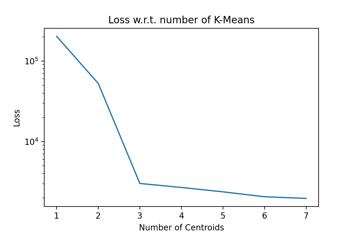
This is a local optimization algorithm. We can restart it multiple times, hoping that it will find a better set of centroid locations, but this is not guaranteed. Usually, this algorithm is restarted to try to get a ‘good’ local minimum. The next immediate question is, ‘How many clusters?’. This is usually data and use-case specific, but if the general rule of thumb is to plot the loss function as a function of the number of clusters. Here an ‘elbow’ or ‘hockey stick’ shape in the graph might inform our choice in the number of clusters. As an example of a plot we would expect to see, I applied k-means on an artificial tri-modal dataset, and we can see the elbow even with a log scale.
Now I want to do something a bit more interesting, image compression via k-Means. We can view the individual pixel colors in an image as a data set. I will apply this to a grayscale image of an iguana for two reasons. There is only 1 dimension in grayscale color data, so visualization is easy, and iguanas are cool.
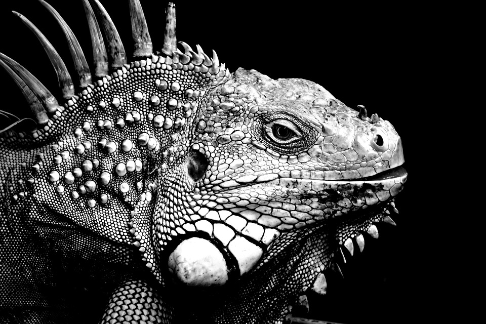
Only small amounts of python were required to read the image and dump the pixel data into a NumPy array.
from PIL import Image
import numpy

# load the image, L tells PIL that this is grayscale
image = Image.open('img.png').convert('L')

# Convert to numpy, flatten then reshape
data = numpy.asarray(image).flatten().reshape(-1,1)

#create bins
bins = [i for i in range(257)]

hist = numpy.histogram(data, bins = bins)
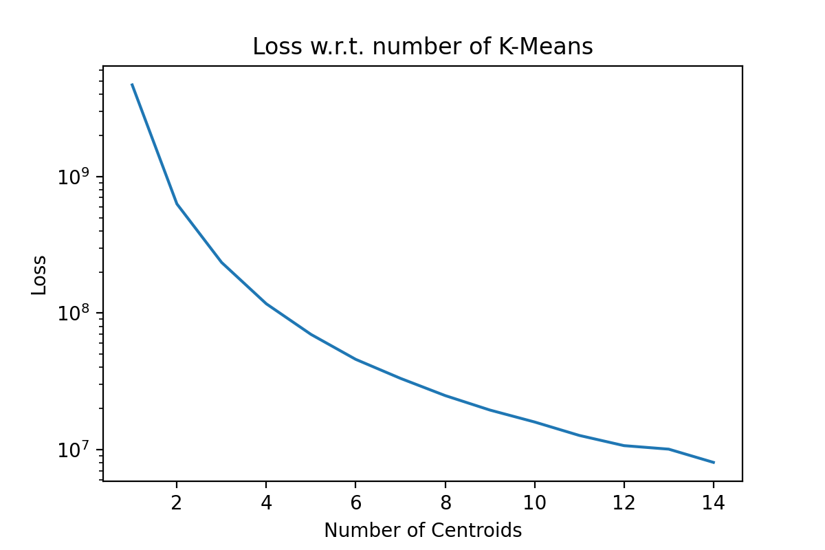
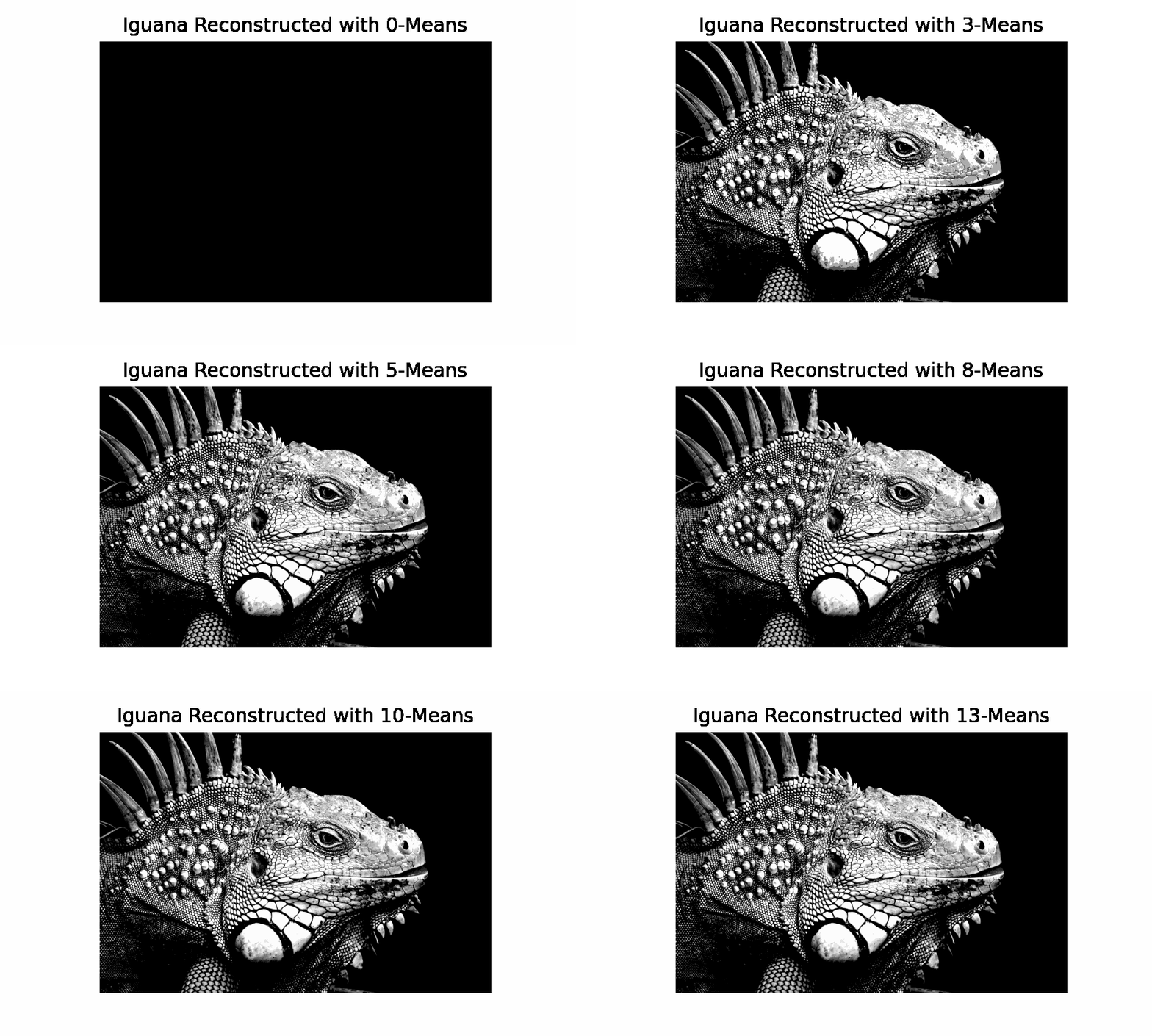
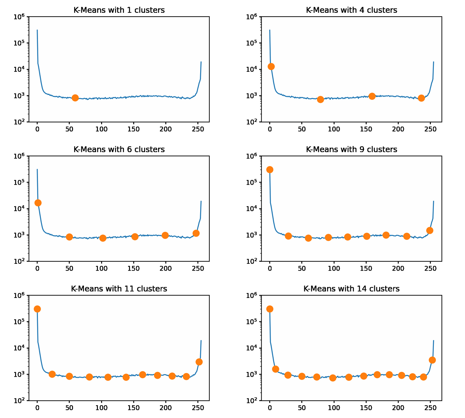
Looking at the iguana data spectrum/histogram, we can clearly see that there are 2 large clusters on the left and right sides of the plot, mapping to black and white in the picture. We can apply k-Means on this data set to get a set of ‘optimal’ pixel values to reconstruct the original image without needing the original dataset. I will be using SKLearn to compute the clusters now, as my slow implementation will 100% not keep up for a data set of approximately 500k data points. I am using the k-means++ initialization and 50 restarts for each cluster count. Here we can use an elbow graph, and we can visually see the image as it is being rebuilt using more and more information. We can see that we start getting depreciating returns after approximately 4 clusters. However, that is not to say that there is not a visual improvement. Reconstructing the image with only 1 cluster is just a single color, so that is quite boring. After only a few clusters being used, we get a very passable result to rebuild Mr.Iguana!
